Does the Box Cox transformation help improve forecasts?

I will rely on the following libraries:

library(data.table)
library(ggplot2)
library(grid)
library(gridExtra)
library(forecast)

## 
## Attache Paket: 'forecast'

## The following object is masked from 'package:ggplot2':
## 
##     autolayer

library(magrittr)
library(future)

The AirPassengers dataset shows the growth in passenger numbers over time on a monthly basis. Let’s create a quick plot comparing the original with the Box Cox transformed dataset. We choose lambda automatically based on minimizing the coefficient of variation (\(\sigma/\mu\)) of the subseries of the Airpassengers series (see Hyndman).

## Original dataset
air_orig = AirPassengers %>%
  autoplot() +
  geom_smooth() +
  ggtitle("Original scale")

## Transformed dataset
AirPassengersBoxCox = BoxCox(AirPassengers, lambda = "auto")

air_box = AirPassengersBoxCox %>%
  autoplot() +
  geom_smooth() +
  ggtitle(paste0("Box Cox with lambda = ", 
                 round(attributes(AirPassengersBoxCox)$lambda,2))
          )
  
## Comparision
grid.arrange(air_orig, air_box, ncol = 2, 
             top = textGrob("Airpassenger numbers over time", 
                            gp = gpar(fontsize = 16))
             )

## `geom_smooth()` using method = 'loess' and formula 'y ~ x'
## `geom_smooth()` using method = 'loess' and formula 'y ~ x'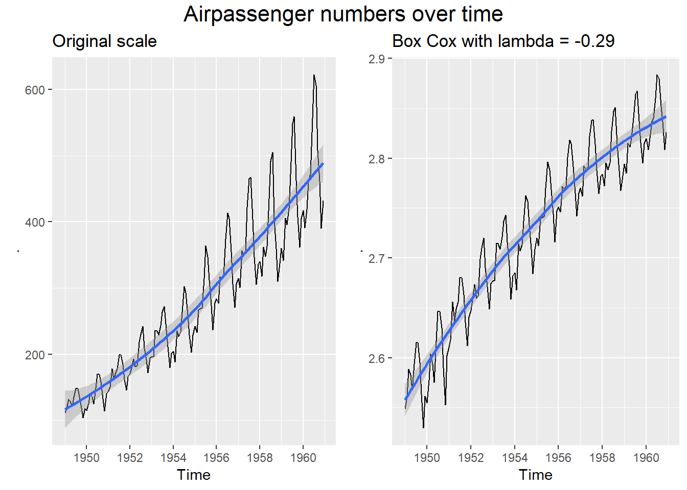

We can clealy see that the original series has a trend and increasing volatility, so it is not stationary. Applying a Box Cox transformation helped us get near constant volatility over the entire time period. We can also see the seasonal pattern of both series.

Let’s quickly look at a histogram to check if the transformation actually helped to make our data more normal:

df_hist = data.frame(passengers = as.double(AirPassengers), type = "Original")

df_hist = rbind(df_hist, data.frame(passengers = as.double(AirPassengersBoxCox), type = "BoxCox"))

ggplot(df_hist, aes(sample = passengers)) +
  geom_qq() +
  geom_qq_line() +
  facet_grid(type ~ ., scales = "free_y") +
  ggtitle("QQ plot: Original and transformed passenger numbers",
          "BoxCox transform did not improve normality markedly")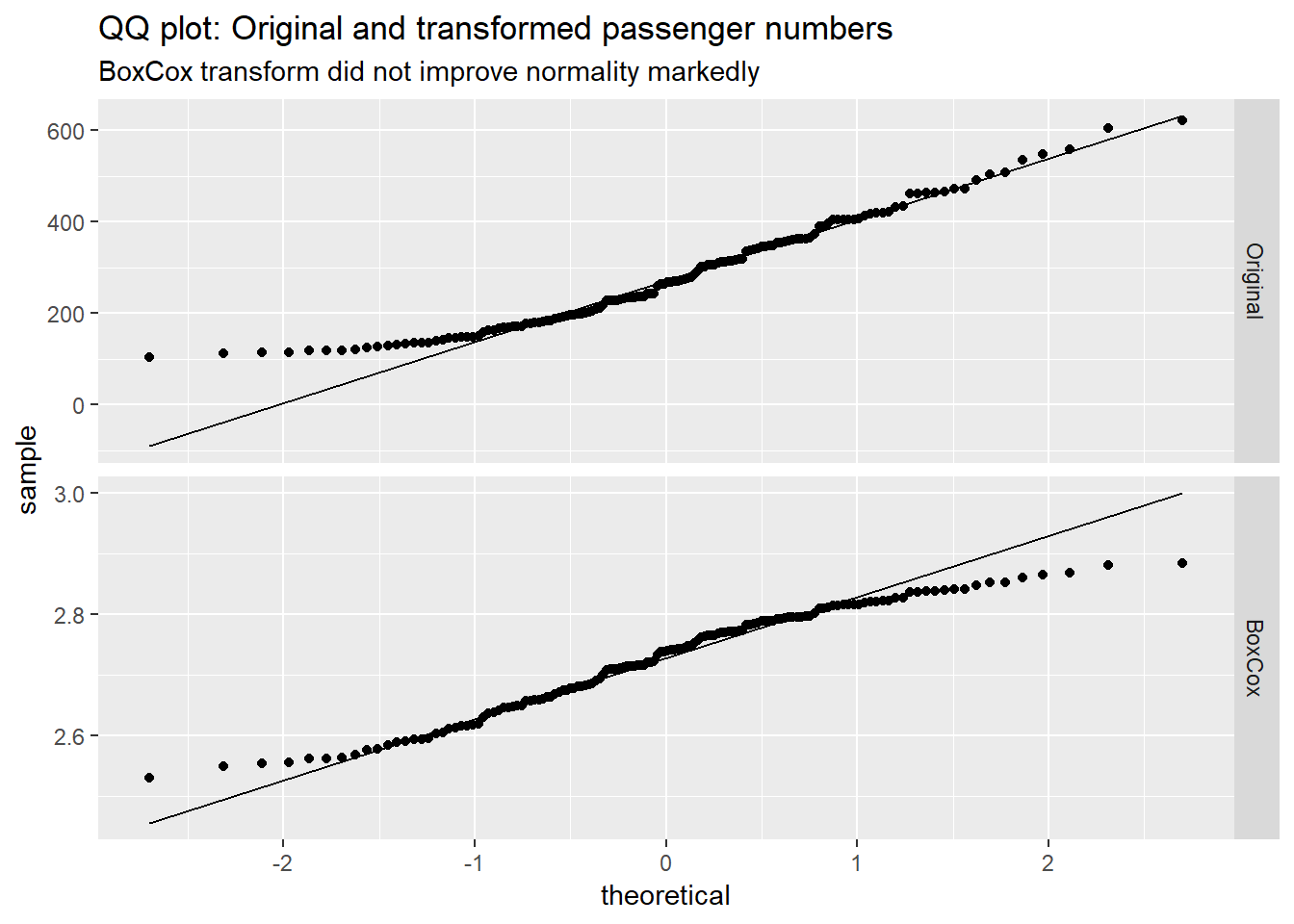

So, while the Box Cox transformation helped to stablize variance, it did not really help a lot with improving normality.

As already mentioned, we are now going to fit two types of models to the series:

• exponential smoothing (ETS) and
• SARIMA models

with and without a Box Cox transformation and see how they compare.

We will start off by training models on all years including 1956 and predicting the following year, i.e. 12 periods ahead to get a feeling for the different models:

AirPassengersTrain = window(AirPassengers, start = c(1949, 1), end = c(1956, 12))
AirPassengersTest = window(AirPassengers, start = c(1957, 1), end = c(1957, 12))

Let’s train the models and create some plots:

plot_arima = forecast(auto.arima(AirPassengersTrain),  h = 12) %>%
  autoplot() + 
  autolayer(AirPassengersTest)

plot_arima_box = forecast(auto.arima(AirPassengersTrain, lambda = "auto", biasadj = T), h = 12) %>%
  autoplot() + 
  autolayer(AirPassengersTest)

grid.arrange(plot_arima, plot_arima_box, ncol = 1, 
             top = textGrob("ARIMA (top) / ARIMA BoxCox (bottom)", 
                            gp = gpar(fontsize = 16)))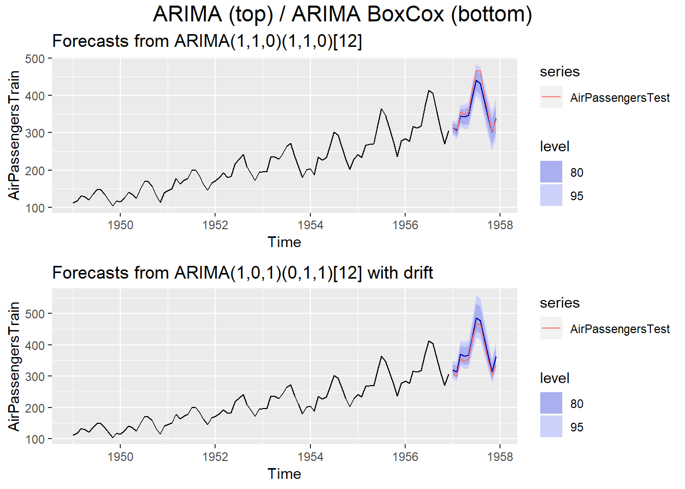

The models picked up on the yearly seasonality in both cases and overall both models perform similarly.

plot_ets = forecast(ets(AirPassengersTrain, allow.multiplicative.trend = T),  
                    h = 12) %>%
  autoplot() + 
  autolayer(AirPassengersTest)

plot_ets_box = forecast(ets(AirPassengersTrain, 
                            allow.multiplicative.trend = T, 
                            lambda = "auto", biasadj = T),  
                        h = 12) %>%
  autoplot() + 
  autolayer(AirPassengersTest)

grid.arrange(plot_ets, plot_ets_box, ncol = 1, 
             top = textGrob("ETS (top) / ETS BoxCox (bottom)", 
                            gp = gpar(fontsize = 16)))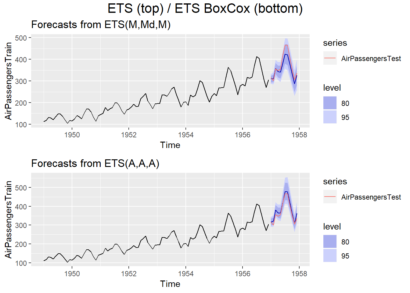

We can see that the vanilla ETS model is performing clearly worse than the ETS-BoxCox version. This suggests that whether a Box Cox transformation helps, depends in large parts on the model in question.

To get a more accurate picture of model performance with(out) Box Cox transformation, we will run a time series cross-validation:

Before we start, we define a few helper functions:

rmse_horizon = function(errors, start = c(1950, 1)) {
  ## removing the first year because of insufficient data
  errors = window(errors, start = start)
  rmse = function(x) sqrt(mean(x^2, na.rm = T))
  
  apply(errors, MARGIN = 2, FUN = rmse)
}

Since the computations take quite some time we will run them async so the current R session is not blocked. We use a ‘multisession’ execution plan, i.e. each core gets to execute one R session in the background. As soon as all cores are busy, evaluation of other futures is blocked.

plan(multisession, workers = 2)

Let’s get started:

## setup
data = AirPassengers
h = 12

##ets
forecastfunction = function(x, h) forecast(ets(x, allow.multiplicative.trend = T), h = h)

rmse_ets  %<-% {
    tsCV(data, forecastfunction = forecastfunction, h = h) %>%
    rmse_horizon()
  }

##ets box
forecastfunction = function(x, h) forecast(ets(x, allow.multiplicative.trend = T, 
                                           lambda = "auto", biasadj = T), h = h)

rmse_ets_box  %<-% {
    tsCV(data, forecastfunction = forecastfunction, h = h) %>%
    rmse_horizon()
  }


##Comparison chart:
rmse_ets_compare = data.frame(rbind(rmse_ets, rmse_ets_box))

rmse_ets_compare %>% 
  cbind(model = c("ets", "ets_box"), .) %>%
  tidyr::gather(key = "h", value = "rmse", 2:13) %>%
  dplyr::mutate(horizon = rep(1:12, each = 2)) %>%
  ggplot(., aes(x = horizon, y = rmse, color = model)) +
  geom_line() +
  ggtitle("RMSE for different forecasting horizons",
         "Box Cox transformation improves forecasts fore most horizons")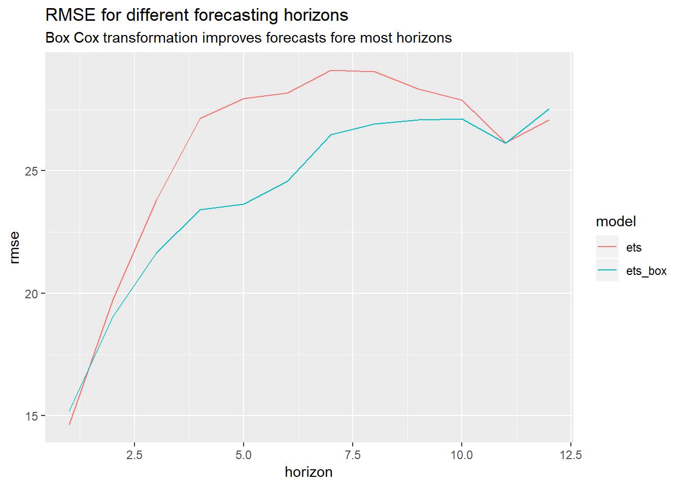

As we can see in the chart above, applying a Box Cox transformation helped to improve performance for most forecasting horizons as we already expected based on the chart in the beginning.

Now let’s try again with SARIMA models:

## setup
data = AirPassengers
h = 12

##arima
forecastfunction = function(x, h) forecast(auto.arima(x), h = h)

rmse_arima  %<-% {
    tsCV(data, forecastfunction = forecastfunction, h = h) %>%
    rmse_horizon()
  }

##arima box
forecastfunction = function(x, h) forecast(auto.arima(x, lambda = "auto", biasadj = T), h = h)

rmse_arima_box  %<-% {
    tsCV(data, forecastfunction = forecastfunction, h = h) %>%
    rmse_horizon()
  }


##Comparison chart:
rmse_arima_compare = data.frame(rbind(rmse_arima, rmse_arima_box))

rmse_arima_compare %>% 
  cbind(model = c("arima", "arima_box"), .) %>%
  tidyr::gather(key = "h", value = "rmse", 2:13) %>%
  dplyr::mutate(horizon = rep(1:12, each = 2)) %>%
  ggplot(., aes(x = horizon, y = rmse, color = model)) +
  geom_line() +
  ggtitle("RMSE for different forecasting horizons",
         "Box Cox transformation gives mixed results")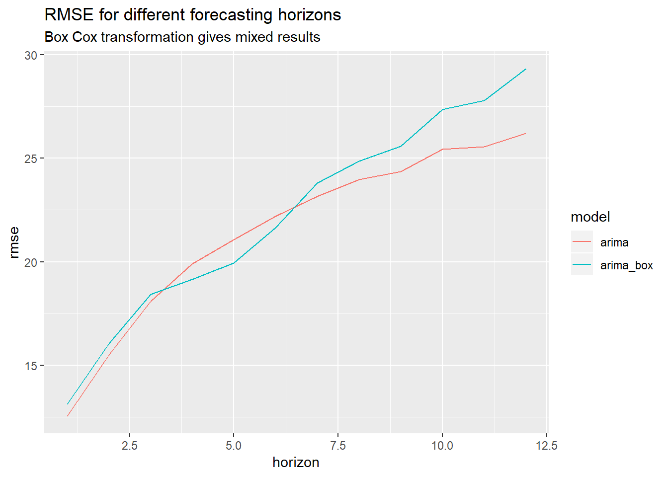

In the SARIMA case, the result is not really clear cut: the Box Cox transformation helps slightly for some time horizons, while making it worse for others. Since there is no clear winner, we stick to the simpler plain-vanilla SARIMA model. Again, this confirms what we saw during our initial exploration in the beginning where ARIMA with(out) Box Cox performed more or less the same.

How does the SARIMA model compare with the Box Cox ETS model?

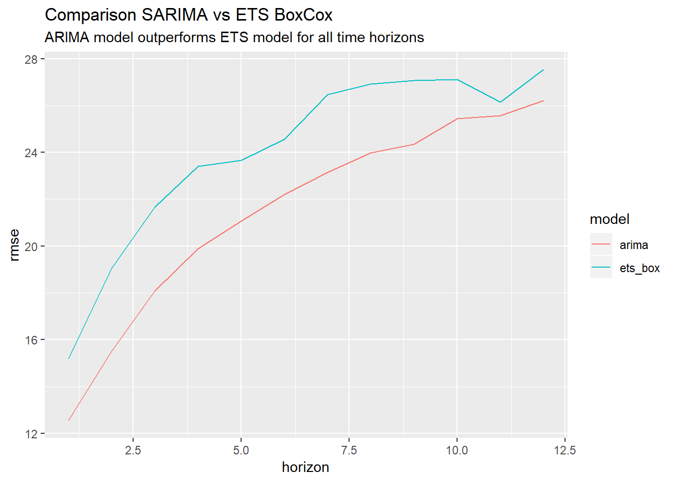
So in this case, a plain vanilla ARIMA model actually works best.

For a final test, let’s add a STL decomposition to our models and see how it affects performance with(out) Box Cox transformation.

STL decomposition in combination with Box Cox transformation

We are now running the same experiment again, but this time we are going to:

1. Apply a STL decomposition,
2. forecast the deseasonalised series after a Box Cox transformation and
3. backtransform and re-seasonalise the data

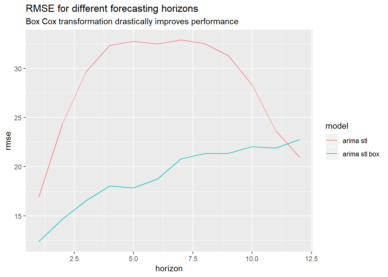
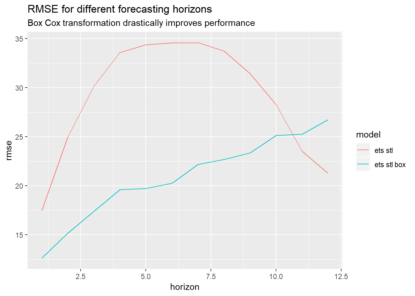
Again, applying a Box Cox transformation helps a lot for most forecasting horizons.

How do the STL with Box Cox perform compared to the plain-vanilla sARIMA model?

rmse_best_arima_ets = data.frame(rbind(rmse_arima, rmse_arima_stl_box, rmse_ets_stl_box))

rmse_best_arima_ets %>% 
  cbind(model = c("arima", "arima_stl_box","ets_stl_box"), .) %>%
  tidyr::gather(key = "h", value = "rmse", 2:13) %>%
  dplyr::mutate(horizon = rep(1:12, each = 3)) %>%
  ggplot(., aes(x = horizon, y = rmse, color = model)) +
  geom_line() +
  ggtitle("Comparison SARIMA vs BoxCox STL+ETS and STL+SARIMA",
         "Box Cox + STL + SARIMA beats other models on all horizons")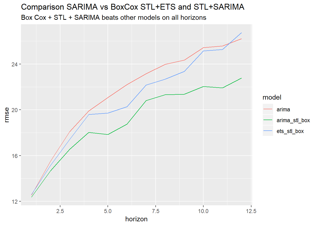

We can see that the combination BoxCox+STL+SARIMA outperforms all other models.

So what is our conclusion? Should we apply a Box Cox transformation or not?

Conclusion

We saw that in certain cases applying a Box Cox transformation can drastically improve performance while in others it decreased performance a bit. The Box Cox transformation really shined in combination with STL.

So to sum up: Box Cox transformations can help with forecasting and should be in every practitioners toolbelt, but with any technique, there is no free-lunch so check your data. As always the answer is: it depends, but based on the experiments it does not seem to hurt much (at least in this case:)

References

Rob Hyndman’s excellent book:

• Forecasting: Principles & Practices, Second Edition

The derivation of the Box Cox Bias correction is based on:

• https://en.wikipedia.org/wiki/Taylor_expansions_for_the_moments_of_functions_of_random_variables
• https://robjhyndman.com/hyndsight/backtransforming

You can find an analytic derivation based on log-normal r.v. here:

• https://davegiles.blogspot.com/2013/08/forecasting-from-log-linear-regressions.html

There is also an interesting section about using transformations to restrict forecasting ranges:

• https://otexts.org/fpp2/transformations.html