Measuring the effect of an intervention on some metric is an important problem in many areas of business and academia. Imagine, you want to know the effect of a recently launched advertising campaign on product sales. In an ideal setting, you would have a treatment and a control group so that you can measure the effect of the campaign. Unfortunately, many times it is not possible or feasible to run a controlled experiment.
This project tries to measure the effect that compulsory wearing of seat belts had on UK driver deaths. We use the ‘SeatBelts’ dataset that contains information on the monthly total of car drivers in the UK killed or seriously injured between January 1969 and December 1984. Using front-seatbelts became mandatory starting 31 January 1983. We are interested in estimating the effect of this law on driver deaths.
To estimate the causal impact, we will try and compare different methods:
- Vanilla Bayesian regression models
- Vanilla model with AR-1 term
- Structural time-series models as implemented in package
CausalImpact
The vanilla regression model is as the name suggests, pretty simple: we simply include an indicator variable equal to 1 starting from the time wearing seatbelts became compulsory and check if the corresponding regression coefficient is statistically different from zero (hopefully negative). Then we extend the model with an AR-1 term and check again. Finally, we use the package CausalImpact to estimate the effect of introducing the seatbelt law.
Setup
This project relies mainly on the following packages:
library(dplyr)
library(tibble)
library(timetk)
library(ggplot2)
library(ggthemes)
library(rstan)
library(rstanarm)
library(CausalImpact)
library(skimr)
Now, let’s load our data set and take a look at some summary statistics:
data_seatbelts = tk_tbl(Seatbelts)

data_seatbelts
## # A tibble: 192 x 9
## index DriversKilled drivers front rear kms PetrolPrice VanKilled
## <S3: ye> <dbl> <dbl> <dbl> <dbl> <dbl> <dbl> <dbl>
## 1 Jan 1969 107. 1687. 867. 269. 9059. 0.103 12.
## 2 Feb 1969 97. 1508. 825. 265. 7685. 0.102 6.
## 3 Mrz 1969 102. 1507. 806. 319. 9963. 0.102 12.
## 4 Apr 1969 87. 1385. 814. 407. 10955. 0.101 8.
## 5 Mai 1969 119. 1632. 991. 454. 11823. 0.101 10.
## 6 Jun 1969 106. 1511. 945. 427. 12391. 0.101 13.
## 7 Jul 1969 110. 1559. 1004. 522. 13460. 0.104 11.
## 8 Aug 1969 106. 1630. 1091. 536. 14055. 0.104 6.
## 9 Sep 1969 107. 1579. 958. 405. 12106. 0.104 10.
## 10 Okt 1969 134. 1653. 850. 437. 11372. 0.103 16.
## # ... with 182 more rows, and 1 more variable: law <dbl>In a next step, we add flags for important safety features that were introduced and split the time index:
data_seatbelts = data_seatbelts %>%
  mutate(month = lubridate::month(data_seatbelts$index),
         year = lubridate::year(data_seatbelts$index),
         time_index = 1:nrow(data_seatbelts),
         eABS = ifelse(year >= 1978, 1, 0),
         airbag = ifelse(year >= 1981, 1, 0)
         ) %>%
  ## Don't forget to convert dummies to factors! (important for model.matrix())
  mutate_at(c("month", "year", "law", "eABS", "airbag"), as.factor)
Before we continue, let’s look at some summary statistics:
overview = skim(data_seatbelts)## Warning: No summary functions for vectors of class: yearmon.
## Coercing to characteroverview## Skim summary statistics
## n obs: 192
## n variables: 14
##
## Variable type: character
## variable missing complete n min max empty n_unique
## index 0 192 192 8 8 0 192
##
## Variable type: factor
## variable missing complete n n_unique top_counts
## airbag 0 192 192 2 0: 144, 1: 48, NA: 0
## eABS 0 192 192 2 0: 108, 1: 84, NA: 0
## law 0 192 192 2 0: 169, 1: 23, NA: 0
## month 0 192 192 12 1: 16, 2: 16, 3: 16, 4: 16
## year 0 192 192 16 196: 12, 197: 12, 197: 12, 197: 12
## ordered
## FALSE
## FALSE
## FALSE
## FALSE
## FALSE
##
## Variable type: integer
## variable missing complete n mean sd p0 p25 p50 p75 p100
## time_index 0 192 192 96.5 55.57 1 48.75 96.5 144.25 192
## hist
## <U+2587><U+2587><U+2587><U+2587><U+2587><U+2587><U+2587><U+2587>
##
## Variable type: numeric
## variable missing complete n mean sd p0 p25
## drivers 0 192 192 1670.31 289.61 1057 1461.75
## DriversKilled 0 192 192 122.8 25.38 60 104.75
## front 0 192 192 837.22 175.1 426 715.5
## kms 0 192 192 14993.6 2938.05 7685 12685
## PetrolPrice 0 192 192 0.1 0.012 0.081 0.093
## rear 0 192 192 401.21 83.1 224 344.75
## VanKilled 0 192 192 9.06 3.64 2 6
## p50 p75 p100 hist
## 1631 1850.75 2654 <U+2582><U+2585><U+2587><U+2585><U+2583><U+2582><U+2581><U+2581>
## 118.5 138 198 <U+2581><U+2583><U+2587><U+2587><U+2585><U+2583><U+2581><U+2581>
## 828.5 950.75 1299 <U+2582><U+2583><U+2585><U+2587><U+2586><U+2585><U+2582><U+2581>
## 14987 17202.5 21626 <U+2581><U+2583><U+2587><U+2587><U+2587><U+2587><U+2585><U+2582>
## 0.1 0.11 0.13 <U+2585><U+2585><U+2583><U+2586><U+2587><U+2587><U+2581><U+2581>
## 401.5 456.25 646 <U+2582><U+2585><U+2586><U+2587><U+2586><U+2583><U+2581><U+2581>
## 8 12 17 <U+2582><U+2586><U+2587><U+2587><U+2586><U+2587><U+2585><U+2581>Some graphs
Before we start the analysis, let’s take a look at the data:
ggplot(data_seatbelts) +
  geom_rect(xmin = 1983.083, xmax = 1984.917,
          ymin = 0, ymax = 0.02,
          fill = tidyquant::palette_light()[[5]],
          alpha = 0.01) +
  geom_line(aes(x = index, y = DriversKilled/kms)) +
  geom_smooth(aes(x = index, y = DriversKilled/kms), method = "lm") +
  geom_line(data = filter(data_seatbelts, law == 1), aes(x = index, y = DriversKilled/kms), col = "blue") +
  geom_vline(xintercept = c(1978, 1981)) +
  annotate("text", x = 1977.2, y = 0.019, label = "eABS") +
  annotate("text", x = 1980.2, y = 0.019, label = "airbag") +
  annotate("text", x = 1983.2, y = 0.019, label = "seatbelt law") +
  theme_hc() +
  ggtitle("# drivers killed/km driven shows declining trend over whole period",
          "Blue line highlights compulsory seatbelt law") +
  xlab(NULL)
## Don't know how to automatically pick scale for object of type yearmon. Defaulting to continuous.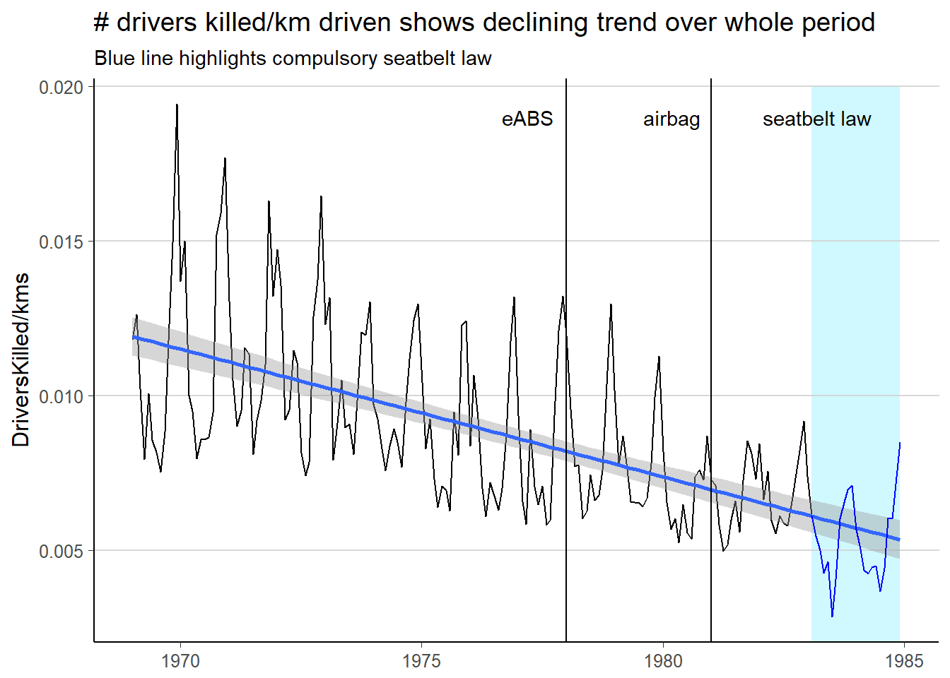
The chart suggests that even before using seatbelts was compulsory, the number of drivers killed per km driven has been declining. So did introducing seatbelts actually help?
Let’s take a quick look at the distribution of DriversKilled/kms:
p_log = ggplot(data_seatbelts, aes(sample = log(DriversKilled) - log(kms))) +
  stat_qq()

p_normal = ggplot(data_seatbelts, aes(sample = DriversKilled/kms)) +
  stat_qq()

gridExtra::grid.arrange(p_normal, p_log, ncol = 2, top = "QQ-Plots: DriversKilled/kms vs. log(DriversKilled/kms) ")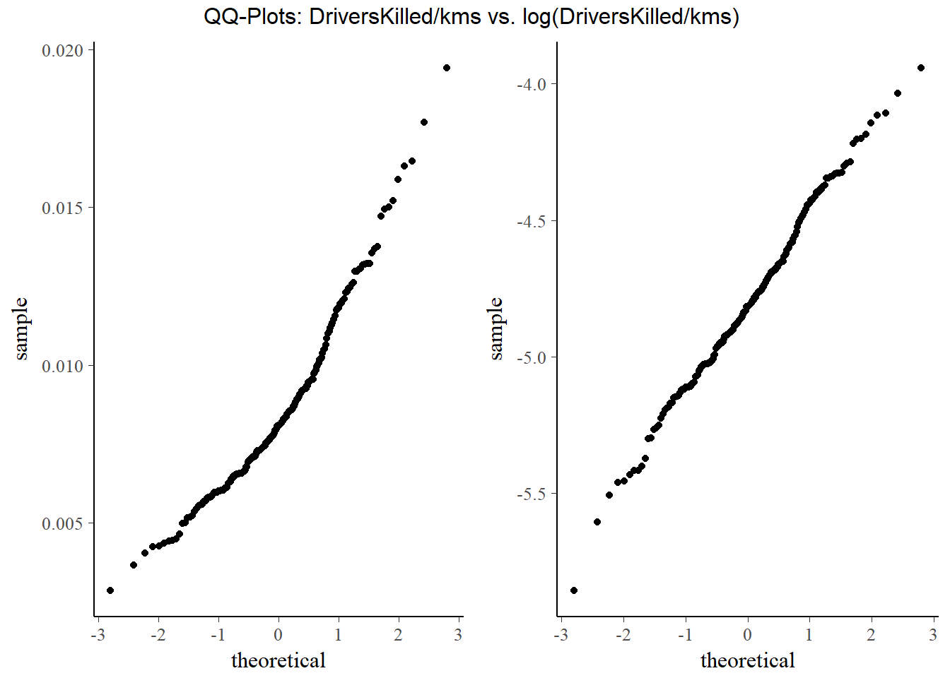
While DriversKilled/kms is not quite normal, the distribution of the log() does not seem to depart much from a normal distribution. While y only needs to be conditionally normal given X, it is quite nice (although not at all necessary!) that it seems to be unconditionally normal too. We will take the log to help with numerical precision. Taking the log also gives a nice interpretation where we have the %-change in number of driver deaths per km driven given our covariates.
We start of by modeling the dependent variable using a vanilla regression model:
Vanilla regression
For the following hand-coded Gibbs sampler we assume the following model:
- observation equation (aka likelihood): \(\textbf{y}|\beta, \sigma \sim \mathcal{N}(\textbf{X}\beta, \sigma^2\textbf{I})\)
- prior distributions: \(\beta|\sigma^2 \sim \mathcal{N}(\textbf{b}_0, \sigma^2\textbf{B}_0)\), \(\sigma^2 \sim \mathcal{IG}(c_0, C_0)\)
By Bayes’ formula, the posterior density is then given by: \[p(\beta, \sigma|y) \sim p(\textbf{y}|\beta, \sigma)p(\beta, \sigma^2) = p(\textbf{y}|\beta, \sigma)p(\beta|\sigma^2)p(\sigma^2)\]
Since a normal-inverse-gamma prior is conjugate to a normal likelihood, the posterior is again a normal-inverse-gamma distribution. So we could either calculate the parameters of the posterior distribution and use it directly or we could use Gibbs sampling to approximate the posterior through simulation. We will do the latter here.
It can be shown that the full conditional distributions of \(\beta\) and \(\sigma\) are given by:
- \(\beta|\textbf{y}, \sigma^2 \sim \mathcal{N}(b_n, B_n)\) with
\[\begin{align*} B_n &= (\frac{1}{\sigma^2}X'X+\frac{1}{\sigma^2}B_0^{-1})^{-1}\\ b_n &= B_n (\frac{1}{\sigma^2}X'y+B_0^{-1}b_0) \end{align*}\] - \(\sigma^2|\textbf{y}, \beta \sim \mathcal{c_n, C_n}\) with
\[\begin{align*} c_n &= c_0 + \frac{n}{2} + \frac{p}{2} \\ C_n &= C_0 + \frac{1}{2}[(y-X\beta)'(y-X\beta) + (\beta - b_0)'B_0^{-1}(\beta-b_0)] \end{align*}\]
This gives us the following vanilla Gibbs sampler:
gibbs_nig = function(y, X, B0_diag = 10^2, b0_mu = 0, c0 = 1, C0 = 1) {
  n = nrow(X)               # no. observations
  p = ncol(X)               # no. predictors incl. intercept

  draws = 10000
  burnin =  1000

  ## initialize some space to hold results:
  res = matrix(as.numeric(NA), nrow=draws+burnin+1, ncol=p+1)
  colnames(res) = c(paste("beta", 0:(p-1), sep='_'), "sigma2")

  ## prior values betas
  B0 = diag(B0_diag, nrow = p, ncol = p)
  b0 = rep(b0_mu, p)

  ## prior values sigma
  C0
  c0

  ## starting values coefficients for sampler
  res[1, ] = rep(1, p+1)

  ## precalculating values
  B0_inv = solve(B0)
  ### (X'X+B0_inv)^(-1)
  pre1 = solve(crossprod(X) + B0_inv)

  ### (X'y + B0_inv*b0)
  pre2 = t(X) %*% y + B0_inv %*% b0

  ### cn = c0 + n/2 + p/2
  cn = c0 + n/2 + p/2

  ## sampling steps
  for (i in 2:(draws+burnin+1)) {
   ## Progress indicator:
   #if (i%%100 == 0) cat("Iteration", i, "done.\n")

   ## beta sampling
    Bn = res[i-1, p+1] * pre1
    bn = Bn %*% (pre2/res[i-1,p+1])
   ## block draw betas:
   res[i,1:p] <- mvtnorm::rmvnorm(1, bn, Bn)

   # draw sigma^2:
   Cn = C0 + .5*(crossprod(y - X %*% res[i, 1:p]) + t(res[i, 1:p] - b0) %*% B0_inv %*% (res[i, 1:p] - b0))
   res[i, p+1] <- 1/rgamma(1, shape = cn, rate = Cn)
  }

  ## throw away initial value and burn-in:
  res = res[-(1:(1000+1)),]

  res
}
Let’s run the sampler and compare the results with a plain OLS estimation:
## running sampler
X = model.matrix(~ PetrolPrice + VanKilled + law + month + time_index, data = data_seatbelts)
y = log(data_seatbelts$DriversKilled) - log(data_seatbelts$kms)

res = gibbs_nig(y, X, B0_diag = 1000, b0_mu = 0)


## posterior mean:
vanilla_bayes = head(colMeans(res), -1)

## OLS estimate:
ols = broom::tidy(lm(log(DriversKilled)-log(kms) ~ PetrolPrice + VanKilled + law + month + time_index, data = data_seatbelts))[1:2]

## prettifying output a bit:
out = cbind(ols, vanilla_bayes, abs(ols$estimate - vanilla_bayes)<0.01)
colnames(out) = c("coeff", "OLS", "Gibbs", "Delta < 0.01")
rownames(out) = NULL
out
## coeff OLS Gibbs Delta < 0.01
## 1 (Intercept) -4.047964950 -4.057938297 TRUE
## 2 PetrolPrice -2.585395621 -2.479176367 FALSE
## 3 VanKilled 0.001267367 0.001225611 TRUE
## 4 law1 -0.135868045 -0.136430294 TRUE
## 5 month2 -0.093704899 -0.093276611 TRUE
## 6 month3 -0.247982128 -0.247318427 TRUE
## 7 month4 -0.294794780 -0.294143484 TRUE
## 8 month5 -0.325415207 -0.324281320 TRUE
## 9 month6 -0.287237168 -0.286592816 TRUE
## 10 month7 -0.364636631 -0.363347731 TRUE
## 11 month8 -0.389147546 -0.388439936 TRUE
## 12 month9 -0.208736279 -0.208575525 TRUE
## 13 month10 -0.035105269 -0.034252927 TRUE
## 14 month11 0.136652145 0.137447998 TRUE
## 15 month12 0.226670664 0.227844203 TRUE
## 16 time_index -0.003399847 -0.003413644 TRUEPretty similar, but not quite the same. Very important to note here is that due to the small sample size (only 192 observations) the priors have quite a strong say on the posterior! If we were to put stronger prior beliefs into our model the prior would dominate the posterior and the results could be very different!
So both models suggest that the introduction of the law actually helped reduce the number of driver deaths per km driven.
Convergence tests
Since the results from our sampler are more or less the same as from OLS, we should not have any convergence issues. Nevertheless, let’s take a look at the traceplots of our parameters:
res_tibble = add_column(as.tibble(res),i = 1:nrow(res), .before = T)

gibbs_gather = tidyr::gather(res_tibble, key = coeff, value = val, 2:17)

ggplot(gibbs_gather, aes(x = i, y = val)) +
  geom_line() +
  facet_grid(coeff ~., scales = "free_y")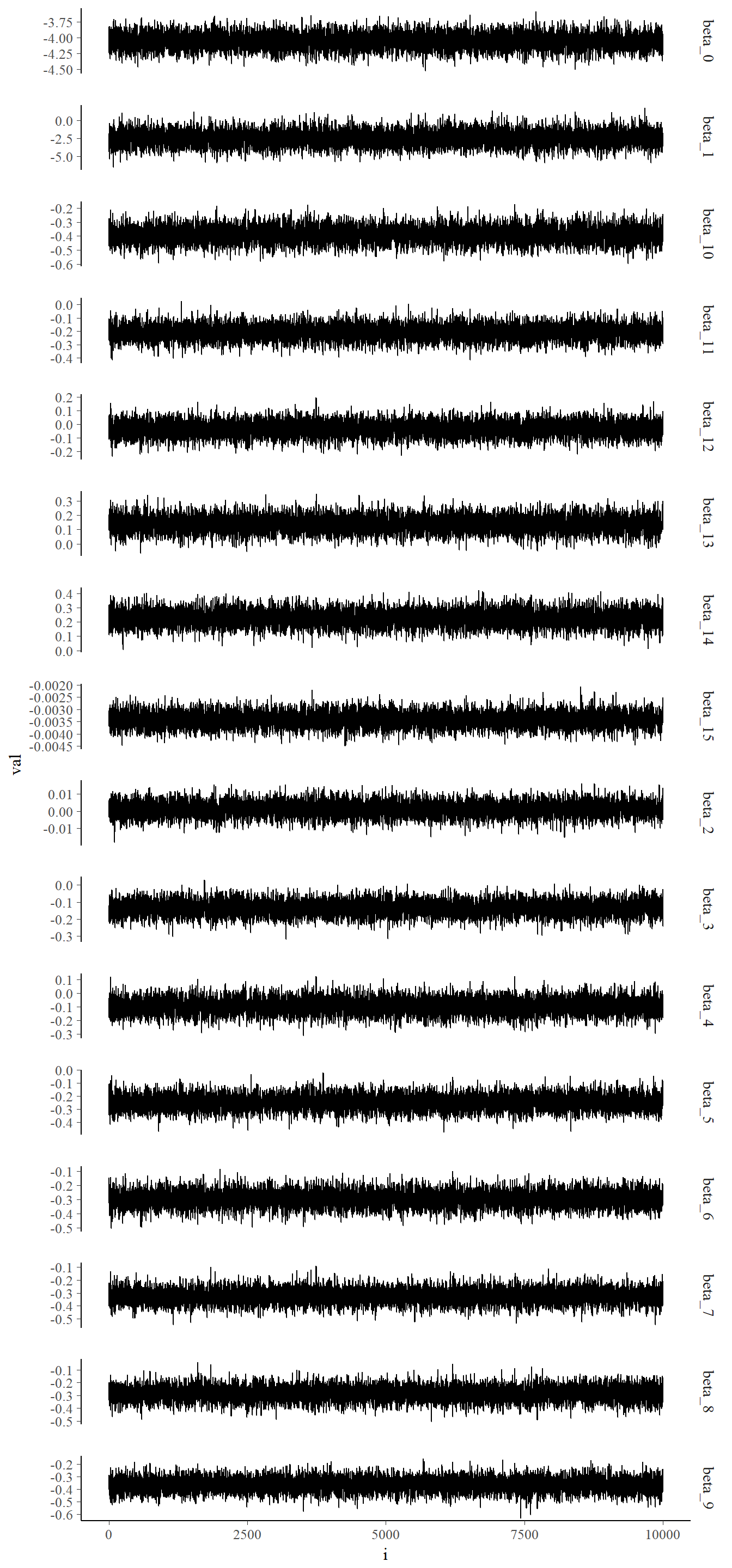
The traceplots show no apparent problems. So our sampler seems to have converged as expected:)
Prior sensitivity tests
In this section we are going to take a look at how strongly our results for the law parameter depend on the prior choice. To do that we are going to look at three cases:
- hard-to-convince case: we are pretty sure that wearing seatbelts and driver deaths are not related:
\[p(law | \sigma^2) \sim \mathcal{N}(0.1, \sigma^2 0.001)\] - undecided case: we are not sure what we should expect (this is the scenario we considered above)
\[p(law | \sigma^2) \sim \mathcal{N}(0, \sigma^2 1000)\] - easy-to-convince case: we are pretty sure that wearing seatbelts is a good idea \[p(law | \sigma^2) \sim \mathcal{N}(-1, \sigma^2 0.01)\]
We will assume a constant prior for \(\sigma^2\) given by \(\sigma^2 \sim \mathcal{IG}(1,1)\) in all cases.
There are again 2 options to get the results: we could either use Gibbs sampling again or we could calculate the posterior distribution of the law coefficient directly. We will stick to using Gibbs sampling, because deriving the marginals analytically is quite messy.
res_h2c = gibbs_nig(y, X, B0_diag = 0.001, b0_mu = 0)
res_e2c = gibbs_nig(y, X, B0_diag = 0.01, b0_mu = -1)

res_h2c_tib = add_column(as.tibble(res_h2c), prior = "hard to convince", i = 1:nrow(res_h2c))
res_e2c_tib = add_column(as.tibble(res_e2c), prior = "easy to convince", i = 1:nrow(res_e2c))
res_undecided = add_column(as.tibble(res), prior = "undecided", i = 1:nrow(res))

temp = bind_rows(res_e2c_tib, res_h2c_tib, res_undecided) %>%
  dplyr::select(beta_3, prior, i)

ggplot(temp, aes(x = beta_3, color = prior)) +
  geom_density() +
  ## intercept OLS
  geom_vline(xintercept = -0.135868045) +
  ggtitle("Prior choice has large impact on resulting posterior",
          "Mainly due to small sample size (N = 192)") +
  xlab("coeff LAW") + ylab("marginal posterior density") +
  theme_hc()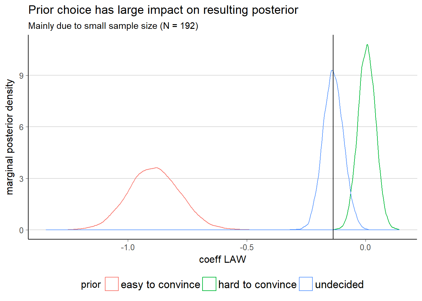
The graph nicely shows that the choice of posterior has quite a large impact. This is mainly due to the fact that we have a small dataset and thus the likelihood does not overcome the prior completely. But while the conclusion in the hard-to-convince case is slightly biased towards no positive influence, we can see that quite a large region is actually still below zero. For this particular example, a prior with a lot of mass on 0, none on positive numbers (because intuitively, wearing a seatbelt should not make you worse off) and a long tail on the left, might be even better for sceptics.
In a next step, we code up the same model, but this time we use Stan to estimate the posterior. First, let’s set some general stan options:
rstan_options(auto_write = TRUE)
options(mc.cores = parallel::detectCores())
As you can see in the model code below, we use the same setup as before, with the same prior values for sigma and beta.
data {
  int<lower=0> N;                         //number of observations
  int<lower=0> K;                         //number of columns (i.e. regressors) in the model matrix
  matrix[N,K] X;                          //model matrix
  vector[N] y;                            //response variable
  real<lower=0> B0_diag;                  //parameters for priors see Gibbs sampler above
  real b0_mu;
  real C0;
  real c0;
}
parameters {
  vector[K] beta;                         //regression parameters - column vector by default
  real<lower=0> sigma;                    //standard deviation
}
model {
  sigma ~ inv_gamma(c0, C0);

  beta ~ normal(b0_mu, sigma*B0_diag);      // coefficients regressors

  y ~ normal(X * beta, sigma);
}
After defining the model, we need to pass our parameters and data to actually sample from it:
# Create model matrix for Stan
X = model.matrix(~ PetrolPrice + VanKilled + law + month + time_index, data = data_seatbelts)
y = log(data_seatbelts$DriversKilled) - log(data_seatbelts$kms)
N = nrow(data_seatbelts)
K = ncol(X)

model_vanilla_test = sampling(vanilla_regression, data = list(N = N, K = K, y = y, X = X,
                                                              B0_diag = 1000, b0_mu = 0, C0 = 1, c0 = 1),
                              chains = 1, cores = 2, iter = 10000, seed = 20170711,
                              control = list(max_treedepth = 10)
                              )
##
## SAMPLING FOR MODEL 'a689d955cfc7fe5b0e8464b346ad79ce' NOW (CHAIN 1).
##
## Gradient evaluation took 0 seconds
## 1000 transitions using 10 leapfrog steps per transition would take 0 seconds.
## Adjust your expectations accordingly!
##
##
## Iteration: 1 / 10000 [ 0%] (Warmup)
## Iteration: 1000 / 10000 [ 10%] (Warmup)
## Iteration: 2000 / 10000 [ 20%] (Warmup)
## Iteration: 3000 / 10000 [ 30%] (Warmup)
## Iteration: 4000 / 10000 [ 40%] (Warmup)
## Iteration: 5000 / 10000 [ 50%] (Warmup)
## Iteration: 5001 / 10000 [ 50%] (Sampling)
## Iteration: 6000 / 10000 [ 60%] (Sampling)
## Iteration: 7000 / 10000 [ 70%] (Sampling)
## Iteration: 8000 / 10000 [ 80%] (Sampling)
## Iteration: 9000 / 10000 [ 90%] (Sampling)
## Iteration: 10000 / 10000 [100%] (Sampling)
##
## Elapsed Time: 11.773 seconds (Warm-up)
## 6.56 seconds (Sampling)
## 18.333 seconds (Total)# pairs(model_vanilla_test)
broom::tidyMCMC(model_vanilla_test, conf.int = T)## term estimate std.error conf.low conf.high
## 1 beta[1] -4.047505982 0.0977261459 -4.236585768 -3.853226699
## 2 beta[2] -2.582375177 0.8657746487 -4.293999388 -0.879935195
## 3 beta[3] 0.001194965 0.0032710143 -0.005154019 0.007618559
## 4 beta[4] -0.135461056 0.0336402519 -0.199438735 -0.069525400
## 5 beta[5] -0.094132437 0.0455087336 -0.182521398 -0.005630879
## 6 beta[6] -0.247948545 0.0448121577 -0.336543204 -0.160019811
## 7 beta[7] -0.294589106 0.0446569692 -0.382885226 -0.209169372
## 8 beta[8] -0.325194648 0.0451775706 -0.415068309 -0.239049761
## 9 beta[9] -0.287410375 0.0445175048 -0.374544704 -0.201934254
## 10 beta[10] -0.363994595 0.0453471439 -0.452265753 -0.275700327
## 11 beta[11] -0.388676229 0.0452666475 -0.479224041 -0.301121033
## 12 beta[12] -0.208374250 0.0450334473 -0.295932642 -0.119991065
## 13 beta[13] -0.034581293 0.0447240080 -0.123050627 0.052973425
## 14 beta[14] 0.137177970 0.0441788607 0.049610912 0.222770939
## 15 beta[15] 0.226935711 0.0437552712 0.139337505 0.314125308
## 16 beta[16] -0.003406782 0.0002431562 -0.003894159 -0.002921927
## 17 sigma 0.124386497 0.0065441175 0.112476042 0.137665693The printed confidence intervals correspond to the 2.5%-97.5% credible interval and the estimate column represents the posterior mean. Fortunately, the results are again very similar to what we got from our first two methods (Note: LAW = beta[4], since I started indexing at 1 in this case, to add to general confusion:)
Stan also offers a formula interface that allows to specify simple models with independence priors and a variance with a flat improper uniform prior on \((0, \infty)\) (correct me if I am wrong, but I think that is the default).
model_glm_vanilla = stan_glm(formula = log(DriversKilled) - log(kms) ~ PetrolPrice + VanKilled +
                               law + month + time_index,
                      data = data_seatbelts,
                      family = gaussian,
                      prior = normal(0,1000),
                      prior_intercept = normal(0,1000),
                      chains = 2,
                      cores = 2,
                      seed = 20170711
                      )

summary(model_glm_vanilla)
##
## Model Info:
##
## function: stan_glm
## family: gaussian [identity]
## formula: log(DriversKilled) - log(kms) ~ PetrolPrice + VanKilled + law +
## month + time_index
## algorithm: sampling
## priors: see help('prior_summary')
## sample: 2000 (posterior sample size)
## observations: 192
## predictors: 16
##
## Estimates:
## mean sd 2.5% 25% 50% 75% 97.5%
## (Intercept) -4.0 0.1 -4.2 -4.1 -4.1 -4.0 -3.9
## PetrolPrice -2.6 0.9 -4.4 -3.2 -2.6 -2.0 -0.8
## VanKilled 0.0 0.0 0.0 0.0 0.0 0.0 0.0
## law1 -0.1 0.0 -0.2 -0.2 -0.1 -0.1 -0.1
## month2 -0.1 0.0 -0.2 -0.1 -0.1 -0.1 0.0
## month3 -0.2 0.0 -0.3 -0.3 -0.2 -0.2 -0.2
## month4 -0.3 0.0 -0.4 -0.3 -0.3 -0.3 -0.2
## month5 -0.3 0.0 -0.4 -0.4 -0.3 -0.3 -0.2
## month6 -0.3 0.0 -0.4 -0.3 -0.3 -0.3 -0.2
## month7 -0.4 0.0 -0.5 -0.4 -0.4 -0.3 -0.3
## month8 -0.4 0.0 -0.5 -0.4 -0.4 -0.4 -0.3
## month9 -0.2 0.0 -0.3 -0.2 -0.2 -0.2 -0.1
## month10 0.0 0.0 -0.1 -0.1 0.0 0.0 0.1
## month11 0.1 0.0 0.1 0.1 0.1 0.2 0.2
## month12 0.2 0.0 0.1 0.2 0.2 0.3 0.3
## time_index 0.0 0.0 0.0 0.0 0.0 0.0 0.0
## sigma 0.1 0.0 0.1 0.1 0.1 0.1 0.1
## mean_PPD -4.8 0.0 -4.8 -4.8 -4.8 -4.8 -4.8
## log-posterior 101.4 3.1 94.6 99.6 101.8 103.6 106.6
##
## Diagnostics:
## mcse Rhat n_eff
## (Intercept) 0.0 1.0 1698
## PetrolPrice 0.0 1.0 2000
## VanKilled 0.0 1.0 2000
## law1 0.0 1.0 2000
## month2 0.0 1.0 1262
## month3 0.0 1.0 1295
## month4 0.0 1.0 1338
## month5 0.0 1.0 1324
## month6 0.0 1.0 1186
## month7 0.0 1.0 1279
## month8 0.0 1.0 1161
## month9 0.0 1.0 1226
## month10 0.0 1.0 1249
## month11 0.0 1.0 1188
## month12 0.0 1.0 1323
## time_index 0.0 1.0 2000
## sigma 0.0 1.0 158
## mean_PPD 0.0 1.0 289
## log-posterior 0.2 1.0 386
##
## For each parameter, mcse is Monte Carlo standard error, n_eff is a crude measure of effective sample size, and Rhat is the potential scale reduction factor on split chains (at convergence Rhat=1).Again, the results are pretty similar, despite the fact that we used independent priors this time. The formula interface from package stanarm offers less choice regarding model specification, but makes up for it by offering a convenient wrapper around Stan that is easy to learn for all R users that are familiar with formulas in lm() and friends.
For the rest of the project we will stick to stanarm to do in-depth analysis.
Model diagnostics
Stan provides an interactive web app for model diagnostics written with the Shiny framework created by the amazing folks at RStudio. Simply call launch_shinystan(<your_fitted_model_here>) to explore diagnostics and model fit statistics.
The rstanarm package is pretty convenient in that it automatically checks whether the chains converge or not. In this case there was no error and a quick check of the trace plots confirms that the chains look pretty good. One possible way to monitor convergence is the Rhat statistic. From the rstanarm vignette: Rhat “…measures the ratio of the average variance of the draws within each chain to the variance of the pooled draws across chains; if all chains are at equilibrium, these will be the same and Rhat will be one. If the chains have not converged to a common distribution, the Rhat statistic will tend to be greater than one.” In our case, Rhat is always 1, so everything appears to be fine.
We will evaluate model fit programmatically. First, let’s see how well the model fits in-sample:
y_rep = posterior_predict(model_glm_vanilla)
dim(y_rep)
## [1] 2000 192We got 2000 simulated points for each observation, in our case 192. Let’s do some plots:
data_plot = as.data.frame(y_rep) %>%
  tidyr::gather(., key = index, value = val, 1:192) %>%
  mutate(index = as.numeric(index)) %>%
  group_by(index) %>%
  summarise(Q0.01 = quantile(val, probs = 0.01),
            mean = mean(val),
            Q0.99 = quantile(val, probs = 0.99)
            )


ggplot(data_plot) +
  ## in-sample prediction
  geom_ribbon(aes(x = index, ymin = Q0.01, ymax = Q0.99), fill = "lightblue") +
  geom_line(aes(x = index, y = mean), col = "blue") +
  ## actual series
  geom_line(data = data_seatbelts, aes(x = time_index, y = log(DriversKilled) - log(kms))) +
  ggtitle("Posterior mean (blue) tracks actual series (black) closely",
          "Ribbon shows Q0.01 - Q0.99 credible interval")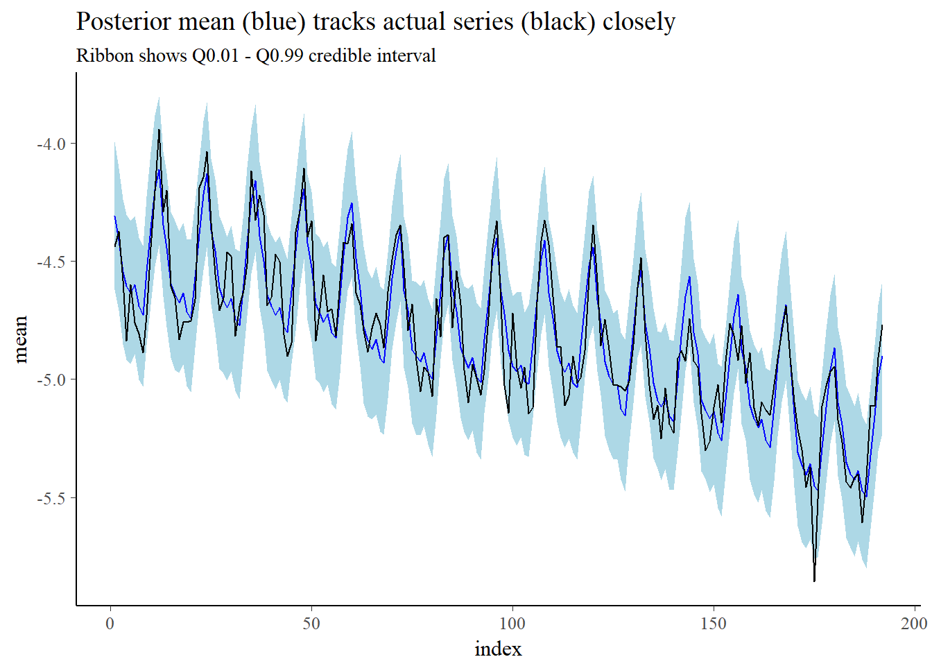
Extending vanilla model
While the model appears to perform quite well, we will nevertheless extend it by allowing first-order serial correlation: \[\begin{align*} Y_t &= \beta_0 + \beta_1 X_{1,t} + \dots + \beta_k X_{k,t} + u_t \\ u_t & = \rho u_{t-1} + v_t,~~v_t \sim \mathcal{N}(0, \sigma^2) \end{align*}\]
Like in the previous section we will start with coding our own Gibbs sampler and then we will implement the model in Stan.
The following derivation closely follows the ‘CCBS Technical Handbook No. 4 - Applied Bayesian econometrics for central bankers’ by Blake and Mumatz (2012) from the Bank of England.
From the model above we can already see that if we knew \(\rho\) than we could get easily get rid of the serial correlation by doing the following: \[\begin{align*} Y_t &= \beta_0 + \beta_1 X_{1,t} + \dots + \beta_k X_{k,t} + u_t \\ - \rho Y_{t-1} &= \rho \beta_0 + \rho \beta_1 X_{1,t-1} + \dots + \rho \beta_k X_{k,t-1} + \rho u_{t-1} \\ \hline \\ Y_t - \rho Y_{t-1} & = \beta_0 (1 - \rho) + \beta_1 (X_{1,t} - X_{1,t-1}) + \dots + \beta_k (X_{k,t} - X_{k,t-1}) + \underbrace{(u_t - u_{t-1})}_{=\epsilon_t} \end{align*}\]
The new model has serially uncorrelated errors. Now we are back in the simple linear regression framework. In other words: the conditional distribution of \(\beta\) coefficients and \(\sigma^2\) is as described in the previous section given that we know \(\rho\).
Now suppose we know the \(\beta\) coefficients. In that case, \(u_t = Y_t - X_t\beta_t\) and we can treat \(u_t = \rho u_t + \epsilon_t\) as a linear regression model in \(\u_t\).
This suggests that our Gibbs sampler should look like this:
- Draw the \(\beta\) coefficients conditional on knowing \(\sigma^2\) and \(\rho\) after serial correlation has been removed
- Afterwards, draw \(\rho\) conditional on \(\beta\) and \(\sigma^2\)
- Finally, conditional on \(\beta\) and \(\rho\), draw \(\sigma\)
For the following hand-coded Gibbs sampler we assume the following model:
- observation equation (aka likelihood): \(\textbf{y}|\beta, \rho, \sigma \sim \mathcal{N}(\textbf{X}\beta + \rho u_{t-1}, \sigma^2\textbf{I})\)
- prior distributions: \(\beta \sim \mathcal{N}(\textbf{b}_0, \textbf{B}_0)\), \(\rho \sim \mathcal{N}(p_n, P_n)\) and \(\sigma^2 \sim \mathcal{IG}(c_0, C_0)\)
Note: This time the prior of \(\beta\) does not depend on \(\sigma^2\) (in contrast to previous Gibbs sampler).
- \(\beta|\textbf{y}, \sigma^2, \rho \sim \mathcal{N}(b_n, B_n)\) with
\[\begin{align} B_n &= \left(\frac{1}{\sigma^2}X'^*X^* + B_0^{-1}\right)^{-1} \\ b_n &= B_n\left(\frac{1}{\sigma^2}X'^*y^* + B_0^{-1}b_0\right) \end{align}\] - \(\rho|\textbf{y}, \beta, \sigma^2 \sim \mathcal{N}(p_n, P_n)\) with
\[\begin{align} P_n &= \left(\frac{1}{\sigma^2}u_{t-1}'u_{t-1} + P_0^{-1}\right)^{-1} \\ p_n &= P_n\left(\frac{1}{\sigma^2}u_{t-1}'u_t + P_0^{-1}p_0\right) \end{align}\] - \(\sigma^2|\textbf{y}, \beta, \rho \sim \mathcal{IG}(c_n, C_n)\) with
\[\begin{align*} c_n &= c_0 + \frac{n}{2} + \frac{p}{2} \\ C_n &= C_0 + \frac{1}{2}[(y^*-X^*\beta)'(y^*-X^*\beta) + (\beta - b_0)'B_0^{-1}(\beta-b_0)] \end{align*}\]
Where \(y_t^* = y_t - \rho y_{t-1}\) and \(X_t^* = X_t - \rho X_{t-1}\).
Using the same priors as in the previous Gibbs sampler would also work, but the estimates of \(\rho\) would be lower on average compared to the estimates you would get when running an ARIMAX model.
gibbs_corr_err <- function(y, X, B0_diag = 10^2, b0_mu = 0, c0 = 0.1, C0 = 0.1, p0 = 0, P0 = 1) {
  n = nrow(X)               # no. observations
  p = ncol(X)               # no. predictors incl. intercept

  draws = 10000
  burnin =  1000

  ## initialize some space to hold results:
  res = matrix(as.numeric(NA), nrow=draws+burnin+1, ncol=p+2)
  colnames(res) = c(paste("beta", 0:(p-1), sep='_'), "sigma2", "rho")

  # define priors
  ## prior values betas
  ### beta ~ normal(b0, B0)
  B0 = diag(B0_diag, nrow = p, ncol = p)
  b0 = rep(b0_mu, p)

  ## prior value sigma
  ### sigma2 ~ IG(c0, C0)
  C0
  c0

  ## prior value rho
  ### rho ~ normal(p0, P0) -> Attention: needs to be corrected later to only allow p in (-1, 1)
  p0
  P0

  ## starting values coefficients for sampler
  ### beta_i = 1, sigma2 = 1, rho = 0
  res[1, ] = c(rep(1, p+1), 0)

  ## precalculating values
  B0_inv = solve(B0)

  ## sampling steps
  for (i in 2:(draws+burnin+1)) {
    ## remove serial correlation
    #i = 2
    rho = res[i-1, p+2]
    sigma2 = res[i-1, p+1]

    y_star = y[-1] - rho*head(y, -1)
    X_star = X[-1, ] - rho*head(X, -1)

    ## beta sampling
    Bn = solve(1/sigma2 * t(X_star) %*% X_star + B0_inv)
    bn = Bn %*%  (1/sigma2 * t(X_star) %*% y_star + B0_inv %*% b0)

    ## block draw betas:
    res[i,1:p] <- mvtnorm::rmvnorm(1, bn, Bn)

    ## rho sampling
    ## calculate model residuals given drawn betas
    u = y - X %*% res[i, 1:p]
    u_L1 = head(u, -1)

    Pn = solve(1/sigma2 * t(u_L1) %*% u_L1 + 1/P0)
    pn = Pn %*% (1/sigma2 * t(u_L1) %*% u[-1] + 1/P0 * p0)

    ## Important: we need to make sure that rho in [-1, 1]
    run = TRUE
    while(run) {
      res[i, p+2] = rnorm(1, pn, Pn)
      run = (res[i, p+2] < -1 | 1 < res[i, p+2])
    }

    ## sigma^2 sampling
    cn = c0 + n/2 + p/2
    Cn = C0 + 0.5 * (crossprod(y_star - X_star %*% res[i, 1:p]) + t(res[i, 1:p] - b0) %*% B0_inv %*% (res[i, 1:p] - b0))
    res[i, p+1] <- 1/rgamma(1, shape = cn, rate = Cn)
  }

  res
}
Let’s try the sampler:
X = model.matrix(~ PetrolPrice + VanKilled + law + month + time_index, data = data_seatbelts)
y = log(data_seatbelts$DriversKilled) - log(data_seatbelts$kms)

res_serial = gibbs_corr_err(y, X)
colMeans(res_serial)
## beta_0 beta_1 beta_2 beta_3 beta_4
## -4.013813641 -2.287443648 -0.001896979 -0.133093040 -0.114328305
## beta_5 beta_6 beta_7 beta_8 beta_9
## -0.266532851 -0.315350748 -0.345077648 -0.302582377 -0.383045366
## beta_10 beta_11 beta_12 beta_13 beta_14
## -0.408607646 -0.227457867 -0.046336094 0.125867092 0.215834683
## beta_15 sigma2 rho
## -0.003500920 0.016327711 0.264551998The coefficients look pretty similar to what we had in the no-autocorrelation sampler, which is reassuring, since autocorrelation should only affect the standard-errors of the coefficients not the coefficients. Let’s compare the results with an ARIMAX model using the same model specification:
## Note: be careful to remove intercept!
X_temp = model.matrix(~ PetrolPrice + VanKilled + law + month + time_index, data = data_seatbelts)[,-1]
y = log(data_seatbelts$DriversKilled) - log(data_seatbelts$kms)

forecast::Arima (y, order=c(0, 0, 1), xreg=X_temp)
## Series: y
## Regression with ARIMA(0,0,1) errors
##
## Coefficients:
## ma1 intercept PetrolPrice VanKilled law1 month2 month3
## 0.2643 -4.0211 -2.4592 -0.0014 -0.1377 -0.1049 -0.2554
## s.e. 0.0735 0.1109 1.0282 0.0031 0.0401 0.0389 0.0435
## month4 month5 month6 month7 month8 month9 month10
## -0.3034 -0.3335 -0.2916 -0.3715 -0.3969 -0.2163 -0.0367
## s.e. 0.0437 0.0436 0.0431 0.0434 0.0435 0.0435 0.0430
## month11 month12 time_index
## 0.1356 0.2233 -0.0035
## s.e. 0.0431 0.0377 0.0003
##
## sigma^2 estimated as 0.01519: log likelihood=138.37
## AIC=-240.73 AICc=-236.78 BIC=-182.1Almost spot on:)
How would this model look like in Stan? We use the same model specification as we did for our hand-coded sampler:
data {
  int<lower=0> N;                         //number of observations
  int<lower=0> K;                         //number of columns (i.e. regressors) in the model matrix
  matrix[N,K] X;                          //model matrix
  vector[N] y;                            //response variable

  //parameters for priors see Gibbs sampler above
  real<lower=0> B0_diag;
  real b0_mu;
  real C0;
  real c0;
  real P0;
  real p0;
}
parameters {
  vector[K] beta;                          //regression parameters - column vector by default
  real<lower=0> sigma;                     //standard deviation
  real<lower=-1, upper=1> rho;             //correlation coefficient error term
}
model {
  real u;
  real rho_scaled;
  sigma ~ inv_gamma(c0, C0);
  rho ~ normal(p0, P0);

  u = 0;

  beta ~ normal(b0_mu, B0_diag);          // coefficients regressors

  for(n in 1:N) {
    y[n] ~ normal(X[n]*beta + u, sigma);      //if a is a matrix, a[m] picks out row m of that matrix

    u = rho * (y[n] - (X[n]*beta));
  }
}
Running the model gives us:
# Create model matrix for Stan
X = model.matrix(~ PetrolPrice + VanKilled + law + month + time_index, data = data_seatbelts)
y = log(data_seatbelts$DriversKilled) - log(data_seatbelts$kms)
N = nrow(data_seatbelts)
K = ncol(X)

model_extended_vanilla = sampling(extended_vanilla_regression, data = list(N = N, K = K, y = y, X = X,
                                                              B0_diag = 1000, b0_mu = 0,
                                                              C0 = 0.1, c0 = 0.1,
                                                              p0 = 0, P0 = 1),
                              chains = 1, cores = 2, iter = 10000, seed = 20170711,
                              control = list(max_treedepth = 10)
                              )
##
## SAMPLING FOR MODEL 'aaa0d39f6a605bd518310da896513842' NOW (CHAIN 1).
##
## Gradient evaluation took 0.001 seconds
## 1000 transitions using 10 leapfrog steps per transition would take 10 seconds.
## Adjust your expectations accordingly!
##
##
## Iteration: 1 / 10000 [ 0%] (Warmup)
## Iteration: 1000 / 10000 [ 10%] (Warmup)
## Iteration: 2000 / 10000 [ 20%] (Warmup)
## Iteration: 3000 / 10000 [ 30%] (Warmup)
## Iteration: 4000 / 10000 [ 40%] (Warmup)
## Iteration: 5000 / 10000 [ 50%] (Warmup)
## Iteration: 5001 / 10000 [ 50%] (Sampling)
## Iteration: 6000 / 10000 [ 60%] (Sampling)
## Iteration: 7000 / 10000 [ 70%] (Sampling)
## Iteration: 8000 / 10000 [ 80%] (Sampling)
## Iteration: 9000 / 10000 [ 90%] (Sampling)
## Iteration: 10000 / 10000 [100%] (Sampling)
##
## Elapsed Time: 71.754 seconds (Warm-up)
## 45.159 seconds (Sampling)
## 116.913 seconds (Total)broom::tidyMCMC(model_extended_vanilla, conf.int = T)## term estimate std.error conf.low conf.high
## 1 beta[1] -4.022969354 0.1272765140 -4.272220157 -3.770700778
## 2 beta[2] -2.406308911 1.1976241927 -4.740874359 0.002743220
## 3 beta[3] -0.001705195 0.0033432738 -0.008207649 0.005009879
## 4 beta[4] -0.137624264 0.0463644869 -0.228658728 -0.043878593
## 5 beta[5] -0.105243197 0.0410217105 -0.183895149 -0.022805223
## 6 beta[6] -0.255652862 0.0440203668 -0.343839752 -0.167714154
## 7 beta[7] -0.304071278 0.0466983734 -0.398088936 -0.211941799
## 8 beta[8] -0.334632210 0.0469710795 -0.426289365 -0.242251880
## 9 beta[9] -0.292132489 0.0458729532 -0.380988679 -0.201737814
## 10 beta[10] -0.372554900 0.0460307607 -0.463595048 -0.284239814
## 11 beta[11] -0.398528276 0.0462730195 -0.489039949 -0.307341672
## 12 beta[12] -0.217816782 0.0464875784 -0.309491862 -0.126817335
## 13 beta[13] -0.037385640 0.0455564180 -0.127708362 0.051927716
## 14 beta[14] 0.134385062 0.0435833417 0.049802748 0.220455952
## 15 beta[15] 0.223289596 0.0391651769 0.147200006 0.300882882
## 16 beta[16] -0.003504902 0.0003094983 -0.004119710 -0.002908423
## 17 sigma 0.124289292 0.0067459748 0.111762019 0.138387908
## 18 rho 0.261100352 0.0752101940 0.112877941 0.405403665The estimates are more or less the same as before so our Stan model should be fine.
# shinystan::launch_shinystan(model_extended_vanilla)
traceplot(model_extended_vanilla, pars = c("beta[4]", "rho")) +
  theme_hc() +
  scale_color_manual(values=c("#CC6666")) +
  ggtitle("Traceplots",
          "No apparent convergence issues")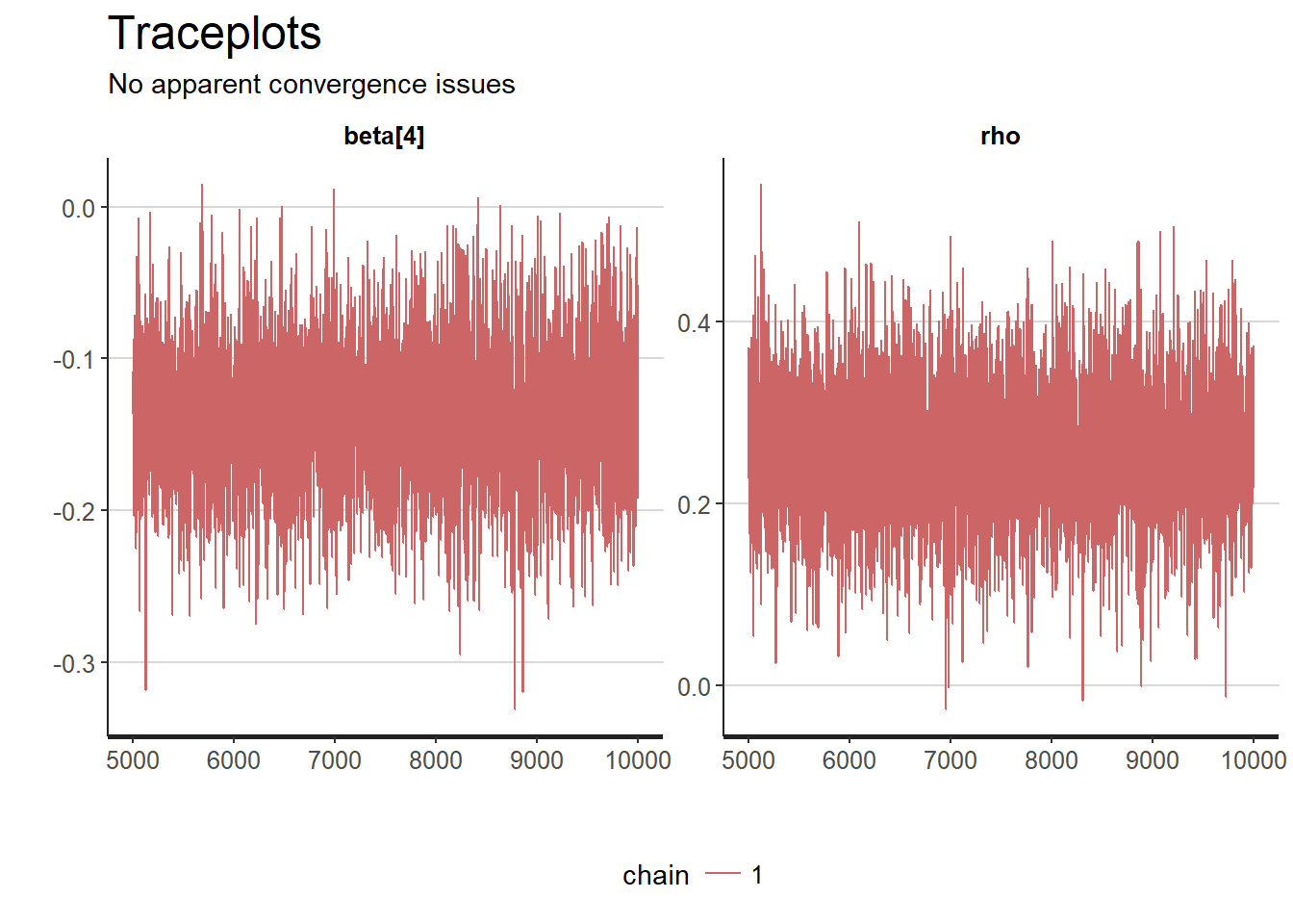
Both chains seem to mix well. So convergence should be fine. Almost all sample points drawn for the LAW coefficient are below 0 so that strengthens our belief that the law did have a positive effect. The distribution of the parameter \(\rho\) is rather wide, suggesting quite some uncertainty, but it is clearly not zero.
Bayesian structural time series models using CausalImpact
In this section we will use yet another approach to check whether the requirement to wear seatbelts helped reduce driver deaths.
Let’s begin by splitting our data set into a pre- and posttreatment phase:
kms = data_seatbelts$kms
drivers = data_seatbelts$drivers
petrol_price = data_seatbelts$PetrolPrice
drivers_killed = data_seatbelts$DriversKilled

time_points = seq.Date(as.Date("1969-01-01"), by = "month", length.out = 192)
pre_period = as.Date(c("1969-01-01", "1983-01-01"))
post_period = as.Date(c("1983-02-01", "1984-12-01"))

data = zoo(cbind(drivers_killed, kms, drivers, petrol_price), time_points)

impact = CausalImpact(data, pre_period, post_period)

impact
## Posterior inference {CausalImpact}
##
## Average Cumulative
## Actual 100 2306
## Prediction (s.d.) 95 (3.3) 2185 (75.4)
## 95% CI [89, 102] [2048, 2343]
##
## Absolute effect (s.d.) 5.3 (3.3) 120.8 (75.4)
## 95% CI [-1.6, 11] [-36.6, 258]
##
## Relative effect (s.d.) 5.5% (3.5%) 5.5% (3.5%)
## 95% CI [-1.7%, 12%] [-1.7%, 12%]
##
## Posterior tail-area probability p: 0.05674
## Posterior prob. of a causal effect: 94%
##
## For more details, type: summary(impact, "report")plot(impact)## Warning: Removed 192 rows containing missing values (geom_path).## Warning: Removed 384 rows containing missing values (geom_path).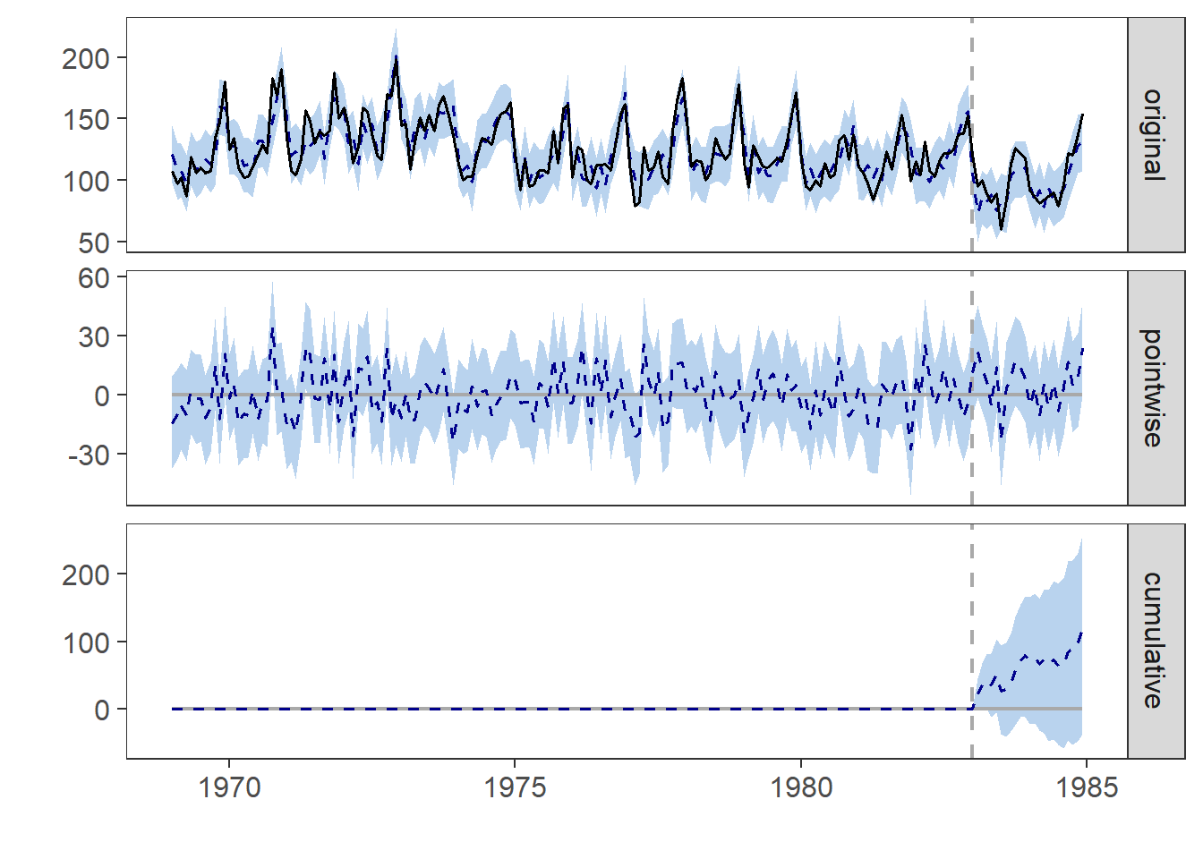
The structural time series model again shows a high likelihood that the introduciton of the seatbelt law helped reduce the number of driver deaths and confirms our previous findings.
I plan to cover using greta, an alternative to stan that uses tensorflow as its backend, for Bayesian inference in some future blog post.
I hope you found this analysis interesting!