Almost every data science course will at some point (usually) sooner than later cover PCA, i.e. Principal Component Analysis. PCA is an important tool used in exploratory data analysis for dimensionality reduction. In this post I want to show you (hopefully in an intuitive way) how PCA works its mathematical magic.
Let’s start with a short description of PCA taken straight from Wikipedia:
PCA is "a statistical procedure that uses an an orthogonal transformation to convert a set of observations of possibly correlated variables into a set of values of linearly uncorrelated variables called principal components. This transformation is defined in such a way that the first principal component […] accounts for as much of the variability in the data as possible, and each succedding component in turn has the highest variance possible under the constraint that it is orthogonal to the preceding components.
So, what does that mean exactly?
Let’s start by looking at a very simple example and take it from there:
library(ggplot2)
library(data.table)

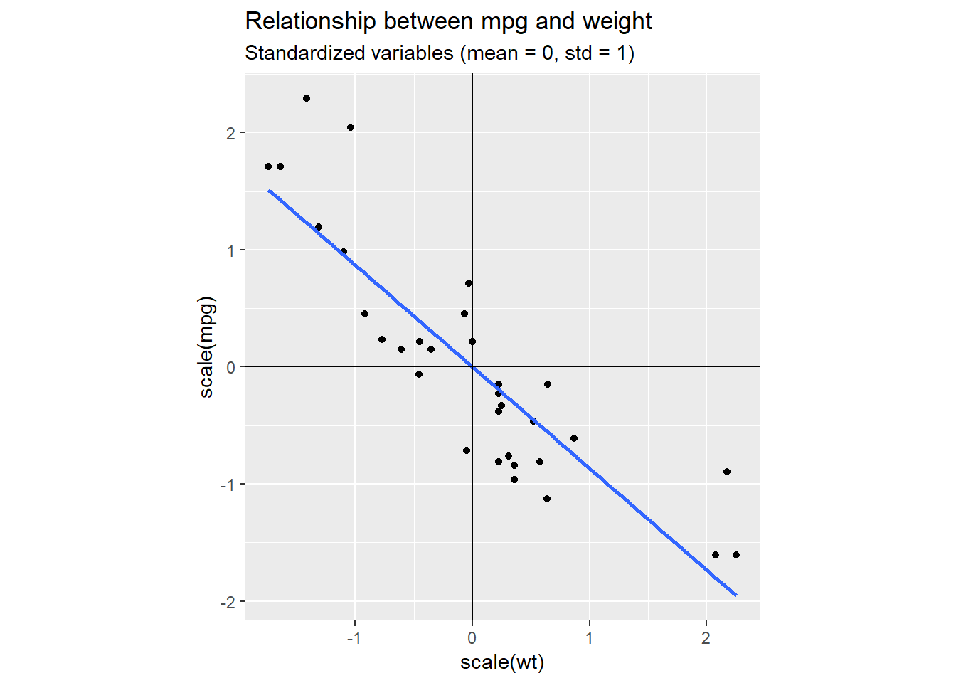
ggplot(mtcars, aes(x = scale(wt), y = scale(mpg))) +
  geom_point() +
  labs(title="Relationship between mpg and weight",
       subtitle="Standardized variables (mean = 0, std = 1)") +
  geom_smooth(method = "lm", se = FALSE) +
  coord_fixed(ratio = 1, xlim = NULL, ylim = NULL, clip = "on")+
  geom_hline(yintercept = 0, color = "black") +
  geom_vline(xintercept = 0, color = "black")
We can clearly see the linear relationship between weight (wt) and miles per gallon (mpg). Most of the points fit rather tightly around the blue line, without deviating to much above or below. So, if we had to summarise our data with one dimension only, it would be quite reasonable to pick a dimension somewhat similar to the blue line. This corresponds to a change in basis. We are rotating our standard basis given by the vectors (1,0) and (0,1) to hopefully find a new basis that better captures the dynamics in our data.
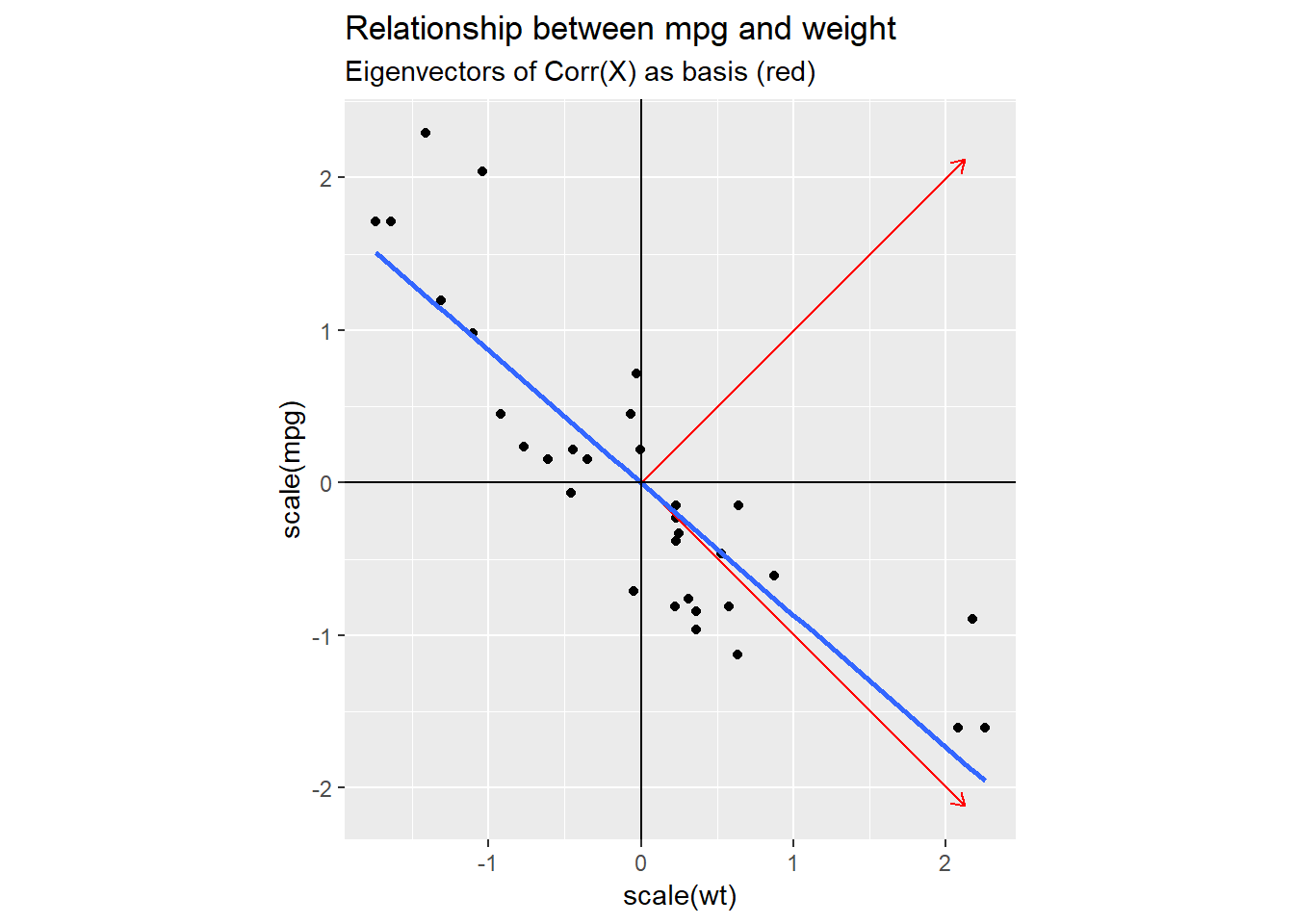
In the next plot, I added one possible new coordinate system (red) that we could use: I set the axis to be equal to the eigenvectors of the covariance matrix of our dataset.

This basis clearly captures the dynamics of our data better than the original one did, but why choose this particular one and not e.g. a coordinate system based on our blue regression line?
Before we continue, let’s take a look at the covariance matrix of mpg and wt.
Remember, a covariance matrix looks like this: \[ Cov(x, y) = \begin{bmatrix} \sigma_x^2 & \sigma_{x,y} \\ \sigma_{y, x} & \sigma_y^2 \end{bmatrix} \] where \(\sigma_{x,y}=\sigma_{y,x}\).
We can easily calculate it using R’s cov function:
cov(mt)## [,1] [,2]
## [1,] 1.0000000 -0.8676594
## [2,] -0.8676594 1.0000000The following exposition is based on the excellent overview of how PCA works by Jon Shlens.
We have already seen in the picture that mpg depends on the weight of the car (the variables covary) which is why the covariance matrix has off-diagonal elements that are not zero. Now imagine we could rotate our coordinate axis so that in the new coordinate system the covariance matrix looks like this: \[ Cov(x, y) = \begin{bmatrix} \sigma_x^2 & 0 \\ 0 & \sigma_y^2 \end{bmatrix} \] The two variables are uncorrelate given our new basis and the axis are aligned with the direction of largest variance so we can easily see which axis is most important to explain the variance in our data.
So given our matrix of observations \(X\), we are looking for a linear transformation matrix \(P\) such that we get a new matrix of observations \(Y\) with a covariance matrix that is diagonal like above:
\[ Y = PX \text{ with } \text{Cov}_Y \text{ diagonal} \]
Let’s start by writing down the matrix expression of the covariance matrix (you might want to take a look at my previous blog post where I summarised some matrix calculation rules): \[ \begin{align} \text{Cov}_Y &= \frac{1}{n-1}YY^t\\ & = \frac{1}{n-1}(PX)(PX)^t \\ & = \frac{1}{n-1} PXX^tP^t \\ & = \frac{1}{n-1} P(XX^t)P^t \\ & = \frac{1}{n-1} PAP^t \end{align} \] We get a new matrix \(A\) which is symmetric by construction. Now we need to brush off our rusty linear algebra knowledge to remember that a symmetric matrix is diagonalized by an orthogonal matrix of its eigenvectors. So we get the following:
\[ A = EDE^t \]
where E is a matrix of eigenvectors of A and D is a diagonal matrix. So if we want to diagonalize \(C_Y\), we need to pick a linear transformation \(P\) = \(E^t\) and use the fact that \(P^{-1}=P^t\) for orthonormal matrices and we get: \[ \begin{align} \text{Cov}_Y &= \frac{1}{n-1}YY^t\\ & = \frac{1}{n-1} PAP^t \\ & = \frac{1}{n-1} PEDE^tP^t \\ & = \frac{1}{n-1} E^tEDE^tE \\ & = \frac{1}{n-1} D \end{align} \] Since we have: \[ P = E^t = E^{-1} \] we see that the eigenvectors form a basis of our transformed space since: \[ Y = E^{-1}X \] is the change of basis from the standard basis to the basis given by \(E\). Since a passive transformation has a corresponding active transformation, we can also view \(P\) as a rotation and a stretch (see Wikipedia for more infos).
So we found the transformation that diagonalizes the covariance matrix \(\text{Cov}_Y\) and that is in a nutshell, what PCA does. We can now select a subset of principal components to reduce the dimension of our dataset. In our particular case we get:
mt = matrix(c(scale(mtcars$wt), scale(mtcars$mpg)), nrow = length(mtcars$mpg), ncol = 2)

eigen_vec = eigen(cov(mt))

eigen_vec
## eigen() decomposition
## $values
## [1] 1.8676594 0.1323406
##
## $vectors
## [,1] [,2]
## [1,] 0.7071068 0.7071068
## [2,] -0.7071068 0.7071068PS: In case you were wondering, why the blue regression line did not correspond to the axis of the first prinicpal component: Regression tries to minimize the distance between the regression line and a point wrt to the y axis (\(\hat{y} - y\)), whereas PCA tries to minimize the orthogonal distance. You can find a few nice graphics illustrating that point here
PPS: Variance is affected by units of measurement, so it is neceassary to first standardize (z-transform) your data before applying PCA. Otherwise ‘large’ variables will naturally account for more variance and distort your analysis.
PPPS: Since PCA is an eigen-decomposition of the covariance matrix (which is mean-centered per definition) mean centering is not necessary, but singular-value-decomposition (svd), a commonly used alternative way to perform PCA, requires centered data. Check out the stackoverflow posts here and here