In this blog post I want to give a brief overview of the core ideas behind the statistical learning framework and show you how to implement a few simple models in this framework.

This post is based on the excellent work “Tree Boosting With XGBoost - Why Does XGBoost Win ‘Every’ machine Learning Competition” by Didrik Nielson.

First, let’s start with some general background info: Statistical learning refers to “learning” patterns from data that generalize well to new incoming data. We can distinguish between two main areas, supervised and unsupervised learning, but in this post I will only focus on the former.

In a supervised learning problem, we have a variable we want to predict (\(y\)) and some covariates, also called features (\(X\)) that might help explain changes in \(y\). Mathematically speaking we have:

\[ \overbrace{\mathcal{D}}^{data set} = \{(y_1, X_{1,1...p}), (y_2, X_{2, 1...p}), ..., (y_n, X_{n,1...p})\} \\ \text{with} \\ y \in \mathcal{Y} \text{ and } X = (X_1, ... X_p) \in \mathcal{X} \] We want to find a function \(f\) that helps us predict \(Y\) given \(X\) with high ‘accuracy’. The function that defines how we measure accuracy is called loss function and our goal is to minimize the expected loss, also know as the risk. The function minimizing risk is called target function and is the function we want to find.

So we have: \[ L: \mathcal{Y} \times \mathcal{A} \to \mathbb{R}_+ \text{... loss function}\\ \text{with}\\ a \in \mathcal{A} \text{... action from set of allowable actions, i.e. a prediction } \hat{y} \]

Some examples include:

• Squared loss: \(L(y, a) = \frac{1}{2}(y - a)^2\)
• Absolute loss: \(L(y, a) = |(y - a)|\)

The risk is now simply the expected value of the loss function: \[ R(a) = \mathbb{E}[L(Y,a)] \] The optimal action \(a^*\) is given by: \[ a^* = \underset{a \in \mathcal{A}}{\text{argmin }} R(a) \]

Note: The argmin operator returns the point where the minimum value is reached, while the min operator returns the value of the function at that point!

To generate predictions \(a\), we use a function, i.e. a model, that maps \(X\) to a: \[ f: \mathcal{X} \to \mathcal{A} \\ a = f(x) \] Where \(\mathcal{A}^{\mathcal{X}}\) is the set of all functions mapping \(\mathcal{X}\) to \(\mathcal{A}\).

The risk of a model is therefore simply: \[ R(f) = \mathbb{E}[L(Y,f(X))] = \mathbb{E}[\mathbb{E}[L(Y, f(X)) | X]] \] by the law of total expectation, with the optimal model given by:

\[ f^* = \underset{f \in \mathcal{A}^{\mathcal{X}}}{\text{argmin }} R(f) \text{ ... target function} \]

This is the function we want to find/estimate. We can calculate the target function pointwise:

\[ f^*(X) =\text{argmin }_{f(x) \in \mathcal{A}^{\mathcal{X}}} \mathbb{E}[L(Y,f(x)) | X = x] \text{ } \forall x \in \mathcal{X} \] Let’s look at the squared loss again. Squared loss risk is given by: \[ R(f) = \mathbb{E}[(Y - f(x))^2 | X = x] \] We can show that the target function is the conditional expectation (see e.g. here for a proof): \[ f^*(x) = \mathbb{E}[Y|X = x] \] and the risk of the target function is given by the conditional variance: \[ R(f^*(x)) = Var[Y | X = x] \]

Since we don’t know the true model risk, we use the empirical risk as a proxy, which is simply an estimate of the true risk: \[ R(\hat{f}) = \frac{1}{n}\sum_{i=1}^nL(y_i, f(x_i)) \\ \text{with} \\ lim_{n \to \infty}R(\hat{f}) = R(f) \text{ by the law of large numbers} \]

So the empirical risk minimizer is given by: \[ \hat{f} = argmin_{f \in \mathcal{F} \subseteq \mathcal{A}^{\mathcal{X}}}R(\hat{f}) \] > Note: We consider only a subspace \(\mathcal{F} \subseteq \mathcal{A}^{\mathcal{X}}\)

Since we only have finitely many datapoints, but an infinite function search space, there are infinitely many functions that fit perfectly in-sample. We thus need to impose additional constraints on our functions, which leads us to consider different model classes:

A model class is nothing more than a restriction \(\mathcal{F} \subseteq \mathcal{A}^{\mathcal{X}}\) of the total function space and is sometimes also called hypothesis space. Each \(mathcal{F}\) can be viewed as a model class. Take for example the class of linear models:

\[ \mathcal{F} = \left\{f: f(x) = \theta_0 + \sum_{i = 1}^p \theta_ixi, \forall x \in \mathcal{X}\right\} \]

To sum up: empirical risk minimization & a given model class turns “learning” into function optimization.

Now, let’s implement linear regression in the statistical learning framework. We want to predict miles per gallon (mpg) using features from the mtcars dataset:

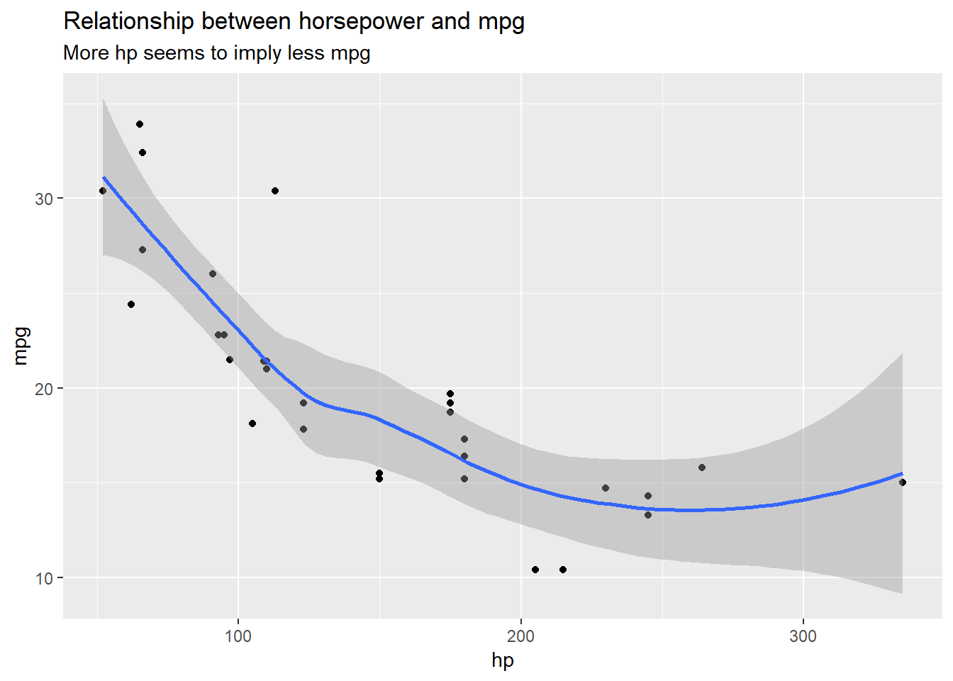
Let’s look at the relation between horsepower (hp) and miles per gallon (mpg):

ggplot(mtcars, aes(x = hp, y = mpg)) +
  geom_point() +
  geom_smooth() +
  labs(title = "Relationship between horsepower and mpg",
       subtitle = "More hp seems to imply less mpg")

## `geom_smooth()` using method = 'loess' and formula 'y ~ x'

Let’s setup our problem using the statistical learning framework:

empirical_risk = function(loss_fun, y, yhat) {
  mean(loss_fun(y, yhat))
}

squared_loss = function(y, yhat) (y - yhat)^2

optim_wrapper = function(params) {
  
  empirical_risk(squared_loss, y = mtcars$mpg, yhat = params[1] + params[2]*mtcars$hp)
  
}

par_loss_sqrt = optim(par = c(0,0), fn = optim_wrapper)
par_loss_sqrt

## $par
## [1] 30.09641090 -0.06821044
## 
## $value
## [1] 13.98982
## 
## $counts
## function gradient 
##       93       NA 
## 
## $convergence
## [1] 0
## 
## $message
## NULL

Let’s compare our output to R’s lm function:

lm(mpg ~ hp, data = mtcars)

## 
## Call:
## lm(formula = mpg ~ hp, data = mtcars)
## 
## Coefficients:
## (Intercept)           hp  
##    30.09886     -0.06823

We get almost the same parameters, which was to be expected, because linear regression or ordinary least squares (OLS) relies on squared loss as the name implies:)

A quick sidenote: In the maximum likelihood setting, we are minimizing \(-log(P(y|X))\), i.e. the density conditional on \(X\). If the density is Gaussian, like in the linear regression setting, we get the squared loss, because the likelihood is given by: \[ Lik(X\beta, \sigma^2|x) = \prod_{i=1}^{n}\frac{1}{\sqrt{2\pi}\sigma}e^{-\frac{(y_i - x_i\beta_i)^2}{2\sigma^2}} \] and applying the \(log\) gives us in essence: \[ (y_i - x_i\beta_i)^2 \]

Now, let’s run the same experiment, with absolute error as a loss function:

absolute_loss = function(y, yhat) abs(y - yhat)

optim_wrapper = function(params) {
  
  empirical_risk(absolute_loss, y = mtcars$mpg, yhat = params[1] + params[2]*mtcars$hp)
  
}

par_loss_abs = optim(par = c(0,0), fn = optim_wrapper)
par_loss_abs

## $par
## [1] 28.13045297 -0.06016883
## 
## $value
## [1] 2.72765
## 
## $counts
## function gradient 
##      265       NA 
## 
## $convergence
## [1] 0
## 
## $message
## NULL

And as theory predicts, parameters change, because our risk minimizer is now the conditional median.

We can also train a non-linear model:

optim_wrapper = function(params) {
  
  empirical_risk(squared_loss, y = mtcars$mpg, yhat = params[1]*exp(params[2]*mtcars$hp))
  
}

set.seed(1234)
par_custom = optim(par = c(0, 0), fn = optim_wrapper, method = "SANN", control = list(maxit = 800000))
par_custom

## $par
## [1] 29.715633368 -0.002983908
## 
## $value
## [1] 13.3925
## 
## $counts
## function gradient 
##   800000       NA 
## 
## $convergence
## [1] 0
## 
## $message
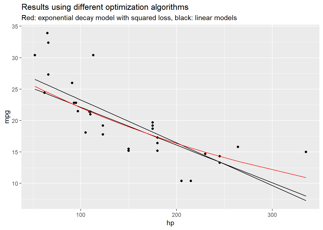
## NULL

Even though this is quite a simple model, just using the default optimization settings as I did before does not cut it anymore. The default algorithms are extremely sensitive to the starting values you pick, but they do work if you take a look at the graph and provide ‘good’ initial guesses. Moreover, since fitting an exponential decay function relys heavily on getting the boundaries correct, a squared loss might be more appropriate than absolute loss as extreme errors are penalized more strongly.

Let’s take a look at the model output:

df_plot = data.frame(mpg = mtcars$mpg, 
                     hp = mtcars$hp,
                     yhat_sqrt = par_loss_sqrt$par[1] + par_loss_sqrt$par[2] * mtcars$hp,
                     yhat_abs = par_loss_abs$par[1] + par_loss_abs$par[2] * mtcars$hp,
                     yhat_cust = par_custom$par[1]*exp(par_custom$par[2] * mtcars$hp)
                    )

ggplot(df_plot, aes(x  = hp, y = mpg)) +
  geom_point() +
  geom_line(aes(y = yhat_sqrt)) + 
  geom_line(aes(y = yhat_abs)) +
  geom_line(aes(y = yhat_cust), color = "red") +
  labs(title = "Results using different optimization algorithms",
       subtitle = "Red: exponential decay model with squared loss, black: linear models")

While the examples above are very simple, the same logics applies to arbitrarily complex problems. In practice, the main problem is finding a good optimizer to solve the optimization problem as we already saw with the last example.

One last sidenote: Terminology in this field can be quite confusing. I was spending quite some time trying to figure out, if I should be talking about objective, loss or cost functions. You can take a look at this stats.stackexchange discussion to see different ways people use these terms in practice. Personally, I like the definition that was accepted as an answer, which goes like this:

• Loss function: defined on a data point and measures the penalty (e.g. squared loss)
• Cost function: usually more general, might be the sum of loss functions over a training set plus some penalty (e.g. MSE)
• Objective function: the most general term for any function that you want to optimize

User lejlot summarises with: > A loss function is a part of a cost function which is a type of an objective function.

But the other definitions are quite nice as well:)

I hope you found my post helpful!