Some Matrix Calculation Rules

Let \(A\), \(B\), \(C\) be \((m \times n)\) matrices and let \(\alpha, \beta \in \mathbb{R}\). Then:

1. \((A + B)^t = A^t + B^t\)
2. \((AB)^t = B^t A^t\)
3. \(A(BC) = (AB)C\)
4. \(A(B + C) = AB + AC\)
5. \((A + B)C = AC + BC\)
6. \(AB \neq BA \text{ in general}\)
7. If \(A, B\) invertible, then:

• \((A^{-1})^{-1} = A\)
• \((A^t)^{-1} = (A^{-1})^t\)
• \((AB)^{-1} = B^{-1}A^{-1}\)

Some Useful Matrix Properties

• Symmetric: A matrix \(A\) is called symmetric \(\iff\) \(A = A^t\)
• Inverse: Matrices \(A, B\) are inverse to each other \(iff\) \(AB = BA = I\). \(A, B\) are called regular or invertible: \(B = A^{-1}\). \(A\) is called singular if it is not invertible
• Let \(A\) be a square matrix. The following are equivalent:
  1. \(A\) is invertible
  2. \(Ax = 0 \iff x = 0\)
  3. The rows/columns of \(A\) are linearly independent

Transformation Matrix

A transformation matrix is the matrix representation of a linear function. If we have a linear transformation: \[ T: \mathbb{R}^n \to \mathbb{R}^m \\ T(x) = y \] we can easily get the matrix representation of \(T\) simply by plugging in our basis vectors: \[ M_T = [T(e_1), \dots, T(e_n)] \in \mathbb{R}^{m, n} \] Let’s look at a simple example. Suppose we have \(T: \mathbb{R}^2 \to \mathbb{R}^2\) with \(T(x, y) = (y, x)^T\). Then we get: \[ M_T^{2, 2} = \begin{bmatrix} 0 & 1 \\ 1 & 0 \end{bmatrix} \]

Representation of Vectors

Taken from my course notes by Prof. Rüdinger Frey:

Let \(x = (x_1, \dots, x_n) \in \mathbb{R}^n\). Then \(x_1, \dots, x_n\) are the (unique) coordinates of \(x\) wrt. the standard basis \(E\): \[ x = x_1 e_1 + \dots + x_n e_n = \sum_{i = 1}^n x_i e_i = E_nx_E \\ \text{ with } \\ x_E = (x_1, \dots, x_n)^T \] If \(B = (b_1, \dots, b_n)\) is another basis of \(\mathbb{R}^n\), then there exist unique numbers \((a_1, \dots, a_n)\) such that x can be written as: \[ x = x_1 b_1 + \dots + x_n b_n = \sum_{i = 1}^n x_i b_i = Bx_B \] We call\((a_1, \dots, a_n)\) the coordinates of x wrt. the basis \(B\) and we write: \[ x_B = \begin{pmatrix} a_1 \\ \vdots \\ a_n \end{pmatrix} \] A basis is simply a set of linearly independent vectors that span a given vector space. the most common basis is called the standard basis \(E\) that we usually work with and that is used in our Cartesian coordinate system. In 2d it looks like this: \[ E_2 = \left\{ \begin{pmatrix} 1 \\ 0 \end{pmatrix}, \begin{pmatrix} 0 \\ 1 \end{pmatrix} \right\} = \{e_1, e_2\} \] So nothing special so far:) Now, let’s take a look at changing our basis, i.e. our coordinate system:

Change of Basis

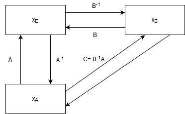
We already saw that we can represent the same vector with different coordinates. Therefore, we can simply write: \[ x = Ex_E = Bx_B \\ \to x_B = B^{-1}Ex_E = B^{-1}x \] So in order to get the coordinates of a vector x wrt. basis B all we have to do is right multiply \(x\) with \(B^{-1}\).

Why does this work? Since a basis is necessarily square and all basis vectors are linearly independent per definition the matrix that represents the basis is invertible.

At university, one of my Profs was quite fond of the following notation: \[ <E, x> = x_E \\ <E, A> = A \\ <B, E> = B^{-1} \] While I did not like it at first, it is quite handy, if you want to quickly write down changes in basis and/or transformations from one vector space to another. All you have to do is make sure that the same letters are next to each other. Let’s look at an example.

Suppose we have a vector v with coordinates wrt. basis \(A\) and we want to transform it to coordinates wrt. basis \(B\):

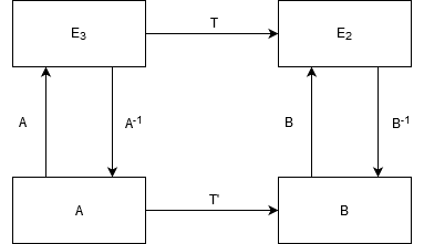
\[ v_B = \overbrace{\underbrace{<B, E>}_{B^{-1}}\underbrace{<E, A>}_{A}}^{C}\underbrace{<A, v>}_{v_A} \] \(C\) is also called the change of basis matrix. The communtative diagram looks as follows: Let’s add a linear transformation to the mix: Suppose we have a vector space with basis \(A\) and another vector space with basis \(B\). There is a linear transformation that maps \(E_n\) to \(E_m\) called \(T\).

How can you find the change of basis matrix that takes you from \(A\) to \(B\)?

\[ v_B = <B, E_m>\underbrace{<E_m, T><T, E_n>}_{T_{E_n, E_m}}<E_n, A><A, v> \] The commutative diagram is the following: Maybe you are wondering:

But why all the fuss about how to change between different basis?

The answer is quite simple: Being able to change the representation of an object can be both computationally handy and offer new insights into the structure of objects.

Changes in basis are also what is called a ‘passive transformation’. While with active transformations we change objects in a given coordinate system (e.g. we rotate or project a vector), with passive transformations we change to coordinate system to get the same effect without changing the object. We merely change its representation. Checkout Wikipedia for some examples.

And last but not least, especially interesting for everyone involved in data analysis: PCA is at its core nothing else than a change in basis such that the coordinate system is rotated to align with the eigenvectors of the covariance matrix, pretty awesome, right?

I plan to write more about PCA in another post.

Hope you found this a little bit helpful.