Python is one if not the most used language by data scientists interested in machine learning and deep learning techniques.
One reason for Python’s popularity is without a doubt scikit-learn. scikit-learn does not need an introduction, but in case you are new to the machine learning space in Python, scikit-learn is an all-in-one machine learning library for Python that implements most machine learning techniques you will need in daily use and provides a consistent api and a framework to work with.
As the name of the post implies, this walk-through is partially intended for users coming from R who already have experience with one or both versions of scikit-learn in the R world, namely caret and mlr3.
So without further ado, let’s get started :)
Survial Chances on the Titanic
For this walk-through I will use one of the most widely used datasets in machine learning: the titanic dataset.
Firstly, because it’s a classic, but more importantely, it is small, readily available and has both numeric, string and missing features. If you want to follow along, you can find the dataset here.
# Load autoreload module
# autoreload 1: reload modules imported with %aimport everytime before execution
# autoreload 2: reload all modules
%load_ext autoreload
%autoreload 2
The autoreload extension is already loaded. To reload it, use:
  %reload_ext autoreload
# Import Libs
import os
import pandas as pd
import numpy as np
import plotly.express as px
from sklearn.impute import SimpleImputer
from sklearn.preprocessing import OneHotEncoder, StandardScaler
from sklearn.pipeline import Pipeline, make_pipeline
from sklearn.compose import ColumnTransformer
from sklearn.model_selection import train_test_split
from sklearn.model_selection import GridSearchCV, cross_val_score
from sklearn.linear_model import LogisticRegression
from sklearn.metrics import roc_auc_score
# # Import dataset
df_titanic = pd.read_csv("../../data/titanic.csv", sep=",", na_values="?")
df_titanic.head()
| pclass | survived | name | sex | age | sibsp | parch | ticket | fare | cabin | embarked | boat | body | home.dest | |
|---|---|---|---|---|---|---|---|---|---|---|---|---|---|---|
| 0 | 1 | 1 | Allen, Miss. Elisabeth Walton | female | 29.0000 | 0 | 0 | 24160 | 211.3375 | B5 | S | 2 | NaN | St Louis, MO |
| 1 | 1 | 1 | Allison, Master. Hudson Trevor | male | 0.9167 | 1 | 2 | 113781 | 151.5500 | C22 C26 | S | 11 | NaN | Montreal, PQ / Chesterville, ON |
| 2 | 1 | 0 | Allison, Miss. Helen Loraine | female | 2.0000 | 1 | 2 | 113781 | 151.5500 | C22 C26 | S | NaN | NaN | Montreal, PQ / Chesterville, ON |
| 3 | 1 | 0 | Allison, Mr. Hudson Joshua Creighton | male | 30.0000 | 1 | 2 | 113781 | 151.5500 | C22 C26 | S | NaN | 135.0 | Montreal, PQ / Chesterville, ON |
| 4 | 1 | 0 | Allison, Mrs. Hudson J C (Bessie Waldo Daniels) | female | 25.0000 | 1 | 2 | 113781 | 151.5500 | C22 C26 | S | NaN | NaN | Montreal, PQ / Chesterville, ON |
So, now that we have our dataframe let’s take a quick look at some summary statistics and plots:
df_titanic.dtypes
pclass         int64
survived       int64
name          object
sex           object
age          float64
sibsp          int64
parch          int64
ticket        object
fare         float64
cabin         object
embarked      object
boat          object
body         float64
home.dest     object
dtype: object
# Note: by default, only numeric attributes are described and NaN values excluded!
df_titanic.describe()
| pclass | survived | age | sibsp | parch | fare | body | |
|---|---|---|---|---|---|---|---|
| count | 1309.000000 | 1309.000000 | 1046.000000 | 1309.000000 | 1309.000000 | 1308.000000 | 121.000000 |
| mean | 2.294882 | 0.381971 | 29.881135 | 0.498854 | 0.385027 | 33.295479 | 160.809917 |
| std | 0.837836 | 0.486055 | 14.413500 | 1.041658 | 0.865560 | 51.758668 | 97.696922 |
| min | 1.000000 | 0.000000 | 0.166700 | 0.000000 | 0.000000 | 0.000000 | 1.000000 |
| 25% | 2.000000 | 0.000000 | 21.000000 | 0.000000 | 0.000000 | 7.895800 | 72.000000 |
| 50% | 3.000000 | 0.000000 | 28.000000 | 0.000000 | 0.000000 | 14.454200 | 155.000000 |
| 75% | 3.000000 | 1.000000 | 39.000000 | 1.000000 | 0.000000 | 31.275000 | 256.000000 |
| max | 3.000000 | 1.000000 | 80.000000 | 8.000000 | 9.000000 | 512.329200 | 328.000000 |
df_titanic.describe(include=[object])
| name | sex | ticket | cabin | embarked | boat | home.dest | |
|---|---|---|---|---|---|---|---|
| count | 1309 | 1309 | 1309 | 295 | 1307 | 486 | 745 |
| unique | 1307 | 2 | 929 | 186 | 3 | 27 | 369 |
| top | Kelly, Mr. James | male | CA. 2343 | C23 C25 C27 | S | 13 | New York, NY |
| freq | 2 | 843 | 11 | 6 | 914 | 39 | 64 |
# Check for NaN values per column
df_titanic.isnull().sum()
pclass          0
survived        0
name            0
sex             0
age           263
sibsp           0
parch           0
ticket          0
fare            1
cabin        1014
embarked        2
boat          823
body         1188
home.dest     564
dtype: int64
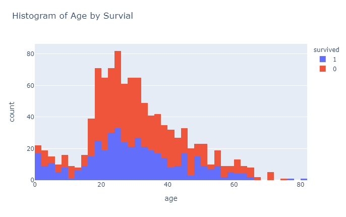
px.histogram(df_titanic, x="age", color = "survived",title="Histogram of Age by Survial")
# Since pandas >0.25 you can aggregate and rename columns in one go:
df_gd = df_titanic.groupby(["sex"], as_index=False). \
                    agg(
                        n_survived=("survived", "sum"),
                        n_sex=("sex", "count")
                       )
# I really like plotly.express, but unfortunately it is not as powerful as ggplot yet
# Converting between discrete and numeric colors for example can only be done by recoding the
# underlying column (https://plotly.com/python/discrete-color/)
df_gd['prop_survived'] = df_gd.n_survived/df_gd.n_sex
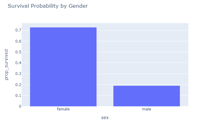
px.bar(df_gd, x = "sex", y="prop_survived", title="Survival Probability by Gender")
So, from these initial plots it seems that being male does not really help your survival chances. Now that we have a rough idea how the dataset looks like, let’s start preparing the data for modeling.
Data Preparation
Unlike R, Python does not have a dataframe as a native data structure which was later provided by the pandas library and nowadays also by datatable. However, when scikit-learn was originally designed in 2007, pandas was not available yet (pandas was first released in 2008). This is probably one of the main reasons why scikit-learn takes some getting used to for R converts who are used to working with dataframes, because scikit-learn expects all inputs in the form of numpy-arrays (though it will automatically convert dataframes as long as they contain only numeric data).
Practically, this used to be a bit of a headache, when you had to work with categorial string data as you needed to transform strings into a numeric representation manually. As a result, there are lots and lots of different tutorials online how to best convert strings to work with scikit-learn.
I will show one way based on pandas and one using scikit-learn. But let’s get rid of some columns first. Passenger name, ticket number and home.dest might be slightly correlated to survivial, but probably not. I don’t know what “boat” and “body” represent and could not find it in the docs, so to make sure we are not accidentally including feature leaks, such as which life boat a person was on, better exclude them.
df_titanic.drop(["name", "ticket", "boat", "body", "home.dest"], axis=1, inplace=True)
# Let's grab only the deck part of the cabin to simplify things:
df_titanic['cabin'] = df_titanic.cabin.astype(str)
df_titanic['cabin'] = df_titanic.cabin.apply(lambda s: s[0])

# cat_vars = df_titanic.columns[df_titanic.dtypes == object].tolist()
cat_vars = ['pclass', 'sex', 'sibsp', 'parch', 'cabin', 'embarked']
num_vars = ['fare', 'age']
# You can also use DataFrame.select_dtypes(...)
# list(df_titanic.select_dtypes(include=['object']).columns)
# 1) get_dummies() from pandas
# Attention: dummy_na = True includes a dummy column even if there are none!
df_m = pd.get_dummies(df_titanic, columns=cat_vars, drop_first=False, dummy_na=True)
Using get_dummies() on a Pandas dataframe can be dangerous when features change between training/test and prediction, because scikit-learn does not know about column names, it only considers column positions!
Let’s use scikit-learn for our encoding:
oh_enc = OneHotEncoder(sparse=False, categories="auto", drop=None, handle_unknown='error')
X_oh = oh_enc.fit_transform(df_titanic[cat_vars])

# OneHotEncoder only includes dummy nan column for columns with nan!
oh_enc.categories_

# Combine numeric and categorical features:
X = np.hstack([df_titanic[num_vars], X_oh])
Using the OneHotEncoder was a bit more work vs. using get_dummies(), but one huge benefit we get is that it integrates neatly into scikit-learns api. Using pipelines, we can do the following:
num_pipeline = Pipeline([('imputer', SimpleImputer(strategy='median')),
                         ('std_scaler', StandardScaler())
                        ])
# Alternatively, a shorter way to construct a pipeline is:
num_pipeline = make_pipeline(SimpleImputer(strategy='median'), StandardScaler())
# Take a look at the pipeline steps:
num_pipeline.steps
# You can access steps by name:
num_pipeline.named_steps["simpleimputer"]

cat_pipeline = Pipeline([('imputer', SimpleImputer(strategy='most_frequent')),
                         ('onehot', OneHotEncoder(sparse=False, handle_unknown="ignore"))
                        ])

preprocessing = ColumnTransformer([('num', num_pipeline, num_vars),
                                   ('cat', cat_pipeline, cat_vars)
                                  ])
# Again, you can use the shortcut: make_column_transformer() similar to make_pipeline()

model_logreg = make_pipeline(preprocessing, LogisticRegression())
A quick note here: If you use a OneHotEncoder in cross-validation, you need to either specify the categories beforehand or allow it to ignore unknown values. Otherwise you will quite likely induce NaNs in your data, because your train folds might not be big enough to contain all categories found in the corresponding test folds.
If you are interested in running feature selection in a pipeline, check out this article from the scikit-learn docs.
y = df_titanic.survived.values
X = df_titanic.drop(["survived"], axis=1)

X_train, X_test, y_train, y_test = train_test_split(X, y, random_state=0)
# Fit the model including the pipeline:
model_logreg.fit(X_train, y_train)
print("Logistic Regression score: {}".format(model_logreg.score(X_test, y_test)))
Logistic Regression score: 0.801829268292683
Pipelines really shine when they are combined with for example grid search, because we can search for the optimal parameters over the entire pipeline:
# By default make_pipeline() uses the lowercased class name as name.
# Again, we can use model_logreg.steps to check the names we have to use:
param_grid = {'columntransformer__num__simpleimputer__strategy': ['median', 'mean'],
              'logisticregression__C': [0.01, 0.1, 1, 10, 100]
             }

grid = GridSearchCV(model_logreg, param_grid, cv=10, scoring='roc_auc', verbose=1, error_score="raise")
grid.fit(X_train, y_train)
grid.best_score_
# Display results table
# pd.DataFrame(grid.cv_results_).T
Fitting 10 folds for each of 10 candidates, totalling 100 fits


0.8416663071613459
Let’s take a quick look at the results from our grid-search:
print("Best estimator:\n{}".format(grid.best_estimator_))
Best estimator:
Pipeline(steps=[('columntransformer',
                 ColumnTransformer(transformers=[('num',
                                                  Pipeline(steps=[('simpleimputer',
                                                                   SimpleImputer()),
                                                                  ('standardscaler',
                                                                   StandardScaler())]),
                                                  ['fare', 'age']),
                                                 ('cat',
                                                  Pipeline(steps=[('imputer',
                                                                   SimpleImputer(strategy='most_frequent')),
                                                                  ('onehot',
                                                                   OneHotEncoder(handle_unknown='ignore',
                                                                                 sparse=False))]),
                                                  ['pclass', 'sex', 'sibsp',
                                                   'parch', 'cabin',
                                                   'embarked'])])),
                ('logisticregression', LogisticRegression(C=1))])
print("Best parameters:\n{}".format(grid.best_params_))
Best parameters:
{'columntransformer__num__simpleimputer__strategy': 'mean', 'logisticregression__C': 1}
print("Best cross-validation score (AUC):{}".format(grid.best_score_))
print("Test set AUC: {}".format(roc_auc_score(y_true=y_test, y_score=grid.best_estimator_.predict(X_test))))
print("Test set best score (default=accuracy): {}".format(grid.best_estimator_.score(X_test, y_test)))
Best cross-validation score (AUC):0.8416663071613459
Test set AUC: 0.775
Test set best score (default=accuracy): 0.801829268292683
# Run the model on our test data with the best pipeline:
print(grid.best_estimator_.predict(X_test)[0:5])
# Return confidence socres for samples:
# From Sklearn docs:
# The confidence score for a sample is the signed distance of that sample to the hyperplane.
print(grid.best_estimator_.decision_function(X_test)[0:5])
[0 1 0 0 0]
[-2.51798632  1.75714031 -1.92149984 -2.26651451 -1.26756091]
Last, but not least, I want to quickly show you how you can easily perform nested-cross-validation:
scores = cross_val_score(
            GridSearchCV(
                model_logreg,
                param_grid,
                cv=10, scoring='roc_auc',
                verbose=1, error_score="raise"),
            X, y)
Fitting 10 folds for each of 10 candidates, totalling 100 fits
Fitting 10 folds for each of 10 candidates, totalling 100 fits
Fitting 10 folds for each of 10 candidates, totalling 100 fits
Fitting 10 folds for each of 10 candidates, totalling 100 fits
Fitting 10 folds for each of 10 candidates, totalling 100 fits
print("Nested cross-validation scores: {}".format(scores))
print("Mean nested-cv-score: {}".format(scores.mean()))
Nested cross-validation scores: [0.8687963  0.78845679 0.70944444 0.74746914 0.73950311]
Mean nested-cv-score: 0.7707339544513457
So, that is about it. I hope this quick walk-through was helpful.
In the beginning I had quite some trouble deciding on a ‘canonic’ way to do things, because there are quite a number of different ways to get to the same end result. I am quite happy with this workflow at the moment, but if you have anys suggestions to improve the workflow, feel free to open a Github issue :)
References
My post follows many recommendations from the book “Introduction to Machine Learning with Python” and only deviates from it significantely when the book I had was not up-to-date (e.g. OneHotEncoder could not handle strings when the book was published)

